BM25 is a short formula, and a working implementation is about thirty lines. The decisions that matter are what to compute in advance, so that query time involves only a few multiplications per posting, and which of several slightly different versions of the formula to compute. Systems that all claim to use "BM25" differ in their IDF, in whether they include a constant factor, in how they store document lengths, and in how they treat repeated query terms. This article gives a compact implementation, traces it by hand on a four-document collection, shows how a document-at-a-time evaluation can skip most of the work while returning the same top results, measures on the Cranfield collection how the two parameters $k_1$ and $b$ affect effectiveness, and measures how much the variants matter.
What to precompute
The BM25 score of document $d$ for query $q$ is
$$\sum_{t \in q} \mathrm{IDF}(t) \cdot \frac{\mathit{tf}_{t,d}\,(k_1 + 1)}{\mathit{tf}_{t,d} + K_d}, \qquad K_d = k_1 \left(1 - b + b\, \frac{L_d}{L_{\mathrm{avg}}}\right).$$
Two parts of this do not depend on the query:
- $\mathrm{IDF}(t)$ depends only on the term and the collection, so it can be stored in the dictionary with each term.
- $K_d$ depends only on the document's length, the average length, and the parameters, so it can be stored in an array indexed by document.
Precomputing both leaves, for each posting $(d, \mathit{tf})$ of each query term, a single expression to evaluate: one addition, one multiplication by the IDF, and one division. The postings must store term frequencies, which an index built only for Boolean retrieval need not (see the inverted index).
Three quantities are easy to get subtly wrong:
- Document length $L_d$ is the number of tokens after analysis (stop words removed, if the index removes them), not the number of distinct terms and not the length of the raw text. Whatever the definition, $L_{\mathrm{avg}}$ must use the same one.
- Document frequency $\mathit{df}$ is the length of the term's postings list, the number of documents containing the term, not its total number of occurrences.
- Both are collection statistics. When documents are added or deleted, $N$, $\mathit{df}$, and $L_{\mathrm{avg}}$ change, and with them every IDF and every $K_d$. Real systems recompute them periodically, or compute them per index segment and accept small inconsistencies.
An implementation
import heapq
import math
from collections import Counter, defaultdict


class BM25Index:
    def __init__(self, docs, k1=1.2, b=0.75):
        """docs: {doc_id: list of analyzed terms}"""
        self.k1, self.b = k1, b
        self.N = len(docs)
        self.postings = defaultdict(list)            # term -> [(doc_id, tf), ...]
        lengths = {}
        for doc_id, terms in docs.items():
            lengths[doc_id] = len(terms)
            for term, tf in Counter(terms).items():
                self.postings[term].append((doc_id, tf))
        avgdl = sum(lengths.values()) / self.N
        # Everything that does not depend on the query is computed once, here.
        self.norm = {d: k1 * (1 - b + b * L / avgdl) for d, L in lengths.items()}
        self.idf = {t: math.log(1 + (self.N - len(p) + 0.5) / (len(p) + 0.5))
                    for t, p in self.postings.items()}

    def search(self, query_terms, k=10):
        scores = defaultdict(float)                  # accumulators, term at a time
        for term in query_terms:
            idf = self.idf.get(term)
            if idf is None:
                continue
            for doc_id, tf in self.postings[term]:
                scores[doc_id] += idf * tf * (self.k1 + 1) / (tf + self.norm[doc_id])
        return heapq.nlargest(k, scores.items(), key=lambda item: item[1])
The scoring loop is the term-at-a-time accumulator method of computing vector scores, with the BM25 term weight in place of the cosine contribution. The IDF uses Lucene's form, which is never negative (see Okapi BM25).
A hand-checked example
Using the four documents from the inverted index and the query juli rise, with $k_1 = 1.2$ and $b = 0.75$. After analysis, the documents are:
| Document | Terms | Length $L_d$ |
|---|---|---|
| 1 | new home sale top forecast | 5 |
| 2 | home sale rise juli | 4 |
| 3 | increas home sale juli | 4 |
| 4 | juli new home sale rise | 5 |
Step 1: what the index stores
Building the index produces, for the two query terms, these postings lists of (document, term frequency) pairs, with the IDF stored beside each term:
| Term | df | IDF | Postings |
|---|---|---|---|
| juli | 3 | $\ln(1 + 1.5/3.5) = 0.3567$ | (2, 1), (3, 1), (4, 1) |
| rise | 2 | $\ln(1 + 2.5/2.5) = 0.6931$ | (2, 1), (4, 1) |
The average length is $(5 + 4 + 4 + 5)/4 = 4.5$, so the stored normalizers are
$$K_d = 1.2\left(0.25 + 0.75 \times \frac{L_d}{4.5}\right) = \begin{cases} 1.1 & L_d = 4 \ (\text{documents 2, 3}) \\ 1.3 & L_d = 5 \ (\text{documents 1, 4}). \end{cases}$$
Each term occurs once where it occurs, so its frequency factor is $\frac{1 \times 2.2}{1 + K_d}$: 1.0476 for the shorter documents and 0.9565 for the longer ones.
Step 2: accumulators, term at a time
The search processes one query term at a time, walking its postings list and adding each document's contribution to that document's accumulator. Accumulators are created on first touch; a document that contains no query term never gets one.
| After processing | Doc 2 | Doc 3 | Doc 4 |
|---|---|---|---|
| juli | $0.3567 \times 1.0476 = 0.3737$ | 0.3737 | $0.3567 \times 0.9565 = 0.3412$ |
| rise | $0.3737 + 0.6931 \times 1.0476 = 1.0998$ | 0.3737 | $0.3412 + 0.6931 \times 0.9565 = 1.0042$ |
Document 1 contains neither term and is never touched. The final step selects the $k$ largest accumulators:
| Rank | Document | Terms matched | Score |
|---|---|---|---|
| 1 | 2 | juli, rise | $(0.3567 + 0.6931) \times 1.0476 = 1.0998$ |
| 2 | 4 | juli, rise | $(0.3567 + 0.6931) \times 0.9565 = 1.0042$ |
| 3 | 3 | juli | $0.3567 \times 1.0476 = 0.3737$ |
The implementation returns exactly these scores (tools/experiments/cranfield/bm25_impl.py prints them, rounded to four decimals). Documents 2 and 4 match the same terms, and length normalization ranks the shorter one first.
Document at a time, with upper bounds
Term-at-a-time scoring needs an accumulator for every document that contains any query term, and it cannot know any document's final score until the last list is read. The alternative, described in computing vector scores, is document-at-a-time evaluation: open every query term's postings list, advance through them together in document order, and finish each document's score when its turn comes. Only the current top $k$ needs to be kept.
Document-at-a-time evaluation makes a further saving possible. BM25's saturation bounds each term's contribution: since $\frac{\mathit{tf}\,(k_1 + 1)}{\mathit{tf} + K_d} < k_1 + 1$ for any frequency, no document can get more than $(k_1 + 1)\,\mathrm{IDF}(t)$ from term $t$. A tighter bound is the largest contribution that actually occurs in the term's postings list, which can be computed once at indexing time. Once the top $k$ is full, its smallest score is a threshold $\theta$, and any document whose bound, the sum of the bounds of the terms it contains, does not exceed $\theta$ cannot enter the top $k$ and need not be scored. This is the principle behind the MaxScore and WAND algorithms (see search at scale).
The example, with $k = 1$
With the bound $(k_1 + 1)\,\mathrm{IDF}$, juli can contribute at most $2.2 \times 0.3567 = 0.7847$ and rise at most $2.2 \times 0.6931 = 1.5249$. Walking the documents in order, keeping only the best one:
| Document | Terms present | Bound | Threshold $\theta$ | Action | Score |
|---|---|---|---|---|---|
| 2 | juli, rise | 2.3096 | 0 | score it | 1.0998, becomes the top 1 |
| 3 | juli | 0.7847 | 1.0998 | skip: bound $\le \theta$ | not computed |
| 4 | juli, rise | 2.3096 | 1.0998 | score it | 1.0042, not better |
Document 3 is never scored, and the answer is the same as before. On four documents the saving is one score; on a real collection it is most of the work.
How much it saves on Cranfield
The Cranfield collection has 1,400 documents, and its queries are long natural-language questions, averaging 11.9 analyzed terms. Term at a time, a query touches on average 2,176 postings and creates 969 accumulators (median 1,027, maximum 1,359), so most queries score most of the collection.
A document-at-a-time evaluation in the style of MaxScore, with exact per-term bounds and $k = 10$, works as follows. Sort the query terms by bound, smallest first. Call the longest run of smallest-bound terms whose bounds add up to no more than $\theta$ the non-essential terms: a document containing only those cannot reach $\theta$, so candidates are drawn only from the postings of the other, essential terms. For each candidate, add the essential terms' contributions, then the non-essential ones in decreasing order of bound, stopping as soon as the partial score plus the remaining bounds falls to $\theta$ or below. As the top 10 fills and $\theta$ rises, more terms become non-essential.
Across the 225 queries this returned the same top 10, in the same order, as exhaustive scoring for every query. It considered 510 candidate documents per query on average and completed the score of 89, which is 9.2 percent of the documents that term-at-a-time scoring scored in full. The saving grows with collection size, because the threshold for the top 10 rises as more good documents are seen, while the number of documents that can beat it stays small.
The effect of $k_1$ and $b$
The defaults $k_1 = 1.2$ and $b = 0.75$ are a starting point. Running the implementation over a grid of values on all 225 Cranfield queries, with the setup of comparing ranking models, shows how much each parameter matters:
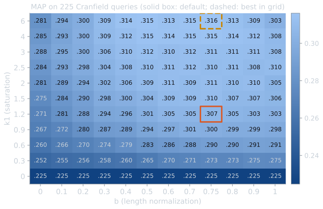
Reading the grid row by row and column by column:
- $k_1 = 0$ discards term frequency. The frequency factor becomes $\mathit{tf}/\mathit{tf} = 1$ for any document containing the term, so BM25 reduces to a sum of IDFs over matching terms, a binary model much like the BIM without relevance information. Its MAP, 0.225, is close to the BIM's 0.220. Every larger $k_1$ does better: term frequency is worth about 0.08 in MAP here.
- $b = 0$ discards length normalization. At $k_1 = 1.2$, MAP falls from 0.307 to 0.271. Cranfield's abstracts vary in length by a factor of more than ten, and without normalization the long ones win too often.
- $b = 1$ normalizes fully and costs a little (0.303 at $k_1 = 1.2$). Full normalization treats all of a long document's length as verbosity, when some long abstracts are long because they cover more, as the BM25 article explains.
- The plateau is broad. Every combination with $k_1$ between 1.2 and 6 and $b$ between 0.5 and 0.9 lies between 0.301 and 0.316. Larger $k_1$, which lets the score keep growing with term frequency for longer before it saturates, helps slightly on this collection.
Measured by nDCG at 10, the picture is the same: 0.368 at the defaults and 0.380 at the best grid point ($k_1 = 6$, $b = 0.5$). Values are rounded to three decimals. This grid was evaluated on all the queries, so its best point is an optimistic estimate of what tuning would achieve on new queries. The comparison article tunes on half the queries and tests on the other half, and finds a gain of 0.003.
Variants that share a name
Kamphuis, de Vries, Boytsov, and Lin (2020) compared eight variants of BM25, drawn from the literature and from widely used systems, on three newswire test collections. The differences among implementations include:
- The IDF. The original Robertson–Spärck Jones form, $\log \frac{N - \mathit{df} + 0.5}{\mathit{df} + 0.5}$, is negative for terms in more than half the collection. Lucene adds 1 inside the logarithm to keep it positive. Others use $\log(N/\mathit{df})$.
- The $(k_1 + 1)$ factor. It scales every score by the same constant and so cannot change a ranking (Robertson and Zaragoza, 2009). Lucene has omitted it since version 8.
- Document length. Some systems store lengths exactly. Lucene stores them in a single byte, with lossy encoding, so documents of somewhat different lengths are normalized identically.
- Repeated query terms. A term appearing twice in the query may be counted twice, counted once, or weighted by a saturated query frequency with the parameter $k_3$. Robertson and Zaragoza (2009) report that the saturation was found unimportant, so counting each occurrence as a separate term is the usual choice.
They found that the differences in effectiveness among the variants were small and that none was statistically significant. The variant still matters for reproducibility, since two papers reporting "BM25" on the same collection can produce different numbers.
How much they matter on Cranfield
Running the variants on the Cranfield collection, with the setup of comparing ranking models, gives a similar picture:
| Variant | MAP | Difference from Lucene form | $p$ |
|---|---|---|---|
| Lucene IDF, with $(k_1 + 1)$, repeated terms counted | 0.3066 | ||
| Original RSJ IDF (can be negative) | 0.3020 | −0.0046 | 0.048 |
| $\log(N/\mathit{df})$ IDF | 0.3065 | −0.0001 | 0.75 |
| Without the $(k_1 + 1)$ factor | 0.3066 | 0 | 1.0 |
| Query terms deduplicated | 0.3063 | −0.0003 | 0.87 |
Removing the constant factor changes nothing, as expected. Only the original IDF makes a measurable difference, and it is small. On Cranfield only one term, flow, occurs in more than half the documents, and its negative weight penalizes documents about the collection's most common subject. On collections where stop-word removal is light, more terms cross the halfway point and the effect can grow. Counting repeated query terms twice, which matters for 66 of the 225 queries, makes no meaningful difference.
Scaling up
The implementation above keeps everything in memory and scores every document that contains any query term. Production systems change three things:
- Compressed postings on disk, decoded as they are read (see index compression).
- Document-at-a-time evaluation with dynamic pruning, as traced above. Methods such as WAND go further than the simple bound check, using the bounds to jump over long stretches of postings lists without decoding them (see computing vector scores and search at scale).
- Precomputed impacts. Some systems store, in place of the term frequency, the term's entire BM25 contribution to the document, quantized to a few bits. Scoring then becomes pure addition, at the cost of fixing $k_1$ and $b$ at indexing time. This site's search box does the same for its instant results: the server precomputes each term's BM25F contribution to each article, and the browser only adds.
For research, toolkits such as Anserini (Yang, Fang, and Lin, 2017), built on Lucene, and its Python interface Pyserini provide BM25 with documented settings and published baselines on standard collections, which makes results reproducible.
References
- Kamphuis, C., de Vries, A. P., Boytsov, L., and Lin, J. (2020). Which BM25 do you mean? A large-scale reproducibility study of scoring variants. In Proceedings of ECIR 2020, 28–34.
- Robertson, S., and Zaragoza, H. (2009). The probabilistic relevance framework: BM25 and beyond. Foundations and Trends in Information Retrieval, 3(4), 333–389.
- Yang, P., Fang, H., and Lin, J. (2017). Anserini: Enabling the use of Lucene for information retrieval research. In Proceedings of SIGIR 2017, 1253–1256.