Suppose the parameters of a controller can be scored only by running it, in a simulator or on a robot, and each run returns a single number. An evolution strategy proposes parameter vectors from a probability distribution, scores them, and moves the distribution toward the better ones. CMA-ES does this with update rules designed one at a time: a weighted mean, an evolution path for the step size, rank-one and rank-μ covariance updates. Natural evolution strategies (NES) derive the update instead, from one principle: treat the expected score of the distribution as a function of the distribution's parameters, and climb it by gradient ascent (Wierstra, Schaul, Peters, and Schmidhuber, 2008; Wierstra et al., 2014). Done naively, that idea is unstable. Done with the natural gradient, it recovers much of CMA-ES, and a stripped-down version of it was used to train neural network policies for reinforcement learning on more than a thousand processors (Salimans, Ho, Chen, Sidor, and Sutskever, 2017).
Search gradients
Let $\pi(\mathbf{z} \mid \theta)$ be a search distribution with parameters $\theta$, for instance a Gaussian with mean $\boldsymbol{\mu}$ and covariance $\Sigma$, and let $f$ be the fitness to be maximized. The expected fitness under the distribution is
$$J(\theta) = \mathrm{E}_\theta[f(\mathbf{z})] = \int f(\mathbf{z})\, \pi(\mathbf{z} \mid \theta)\, d\mathbf{z}.$$
Its gradient with respect to $\theta$ does not require the gradient of $f$. Moving the derivative inside the integral and multiplying and dividing by $\pi$ gives the log-likelihood trick:
$$\nabla_\theta J(\theta) = \int f(\mathbf{z})\, \nabla_\theta \pi(\mathbf{z} \mid \theta)\, d\mathbf{z} = \mathrm{E}_\theta\bigl[f(\mathbf{z})\, \nabla_\theta \log \pi(\mathbf{z} \mid \theta)\bigr].$$
Step by step, and with the reason for each step:
- $\nabla_\theta J = \nabla_\theta \int f(\mathbf{z})\,\pi(\mathbf{z} \mid \theta)\,d\mathbf{z} = \int f(\mathbf{z})\,\nabla_\theta \pi(\mathbf{z} \mid \theta)\,d\mathbf{z}$. Only $\pi$ depends on $\theta$; $f$ is evaluated at fixed points $\mathbf{z}$. Exchanging derivative and integral is allowed for the smooth densities used here when $f$ is integrable, and it is the only place where $f$ meets the derivative, which is why $f$ itself need not be differentiable or even continuous.
- $\nabla_\theta \pi = \pi\, \nabla_\theta \log \pi$, the chain rule for the logarithm read backwards.
- Substituting gives $\int f(\mathbf{z})\,\nabla_\theta \log \pi(\mathbf{z} \mid \theta)\,\pi(\mathbf{z} \mid \theta)\,d\mathbf{z}$, which is an expectation under the current distribution, so it can be estimated by sampling from that distribution, the one thing an evolution strategy does anyway.
The term $\nabla_\theta \log \pi$ is called the score. It has mean zero, since $\mathrm{E}[\nabla_\theta \log \pi] = \int \nabla_\theta \pi\, d\mathbf{z} = \nabla_\theta \int \pi\, d\mathbf{z} = \nabla_\theta 1 = 0$. Consequently any constant $b$ can be subtracted from $f$ without changing the expected gradient, $\mathrm{E}[(f - b)\nabla_\theta \log \pi] = \mathrm{E}[f\,\nabla_\theta \log \pi]$, and a well-chosen $b$ greatly reduces the variance of the estimate. This baseline reappears below as the zero sum of the fitness-shaping utilities and as antithetic sampling.
The expectation can be estimated from a population of $\lambda$ samples, $\nabla_\theta J \approx \frac{1}{\lambda} \sum_{k=1}^{\lambda} f(\mathbf{z}_k) \nabla_\theta \log \pi(\mathbf{z}_k \mid \theta)$, and the parameters updated by $\theta \leftarrow \theta + \eta \nabla_\theta J$ with a learning rate $\eta$. Wierstra et al. (2014, §2) call this a search gradient: the population is no longer a set of individuals that survive or die, but a sample used to estimate a direction in the space of distributions. Salimans et al. (2017) note that it is the score function estimator, used in a fashion similar to REINFORCE (Williams, 1992), but applied to the parameters of the search distribution rather than to a policy's actions.
For a Gaussian the log-derivatives are simple. With $\mathbf{z} \sim \mathcal{N}(\boldsymbol{\mu}, \Sigma)$,
$$\nabla_{\boldsymbol{\mu}} \log \pi = \Sigma^{-1}(\mathbf{z} - \boldsymbol{\mu}), \qquad \nabla_{\Sigma} \log \pi = \tfrac{1}{2}\Sigma^{-1}(\mathbf{z} - \boldsymbol{\mu})(\mathbf{z} - \boldsymbol{\mu})^\top \Sigma^{-1} - \tfrac{1}{2}\Sigma^{-1}.$$
Samples with high fitness pull the mean toward themselves and stretch the covariance in their direction.
Why the plain gradient fails
Take one dimension, $z \sim \mathcal{N}(\mu, \sigma^2)$, and write $s = (z - \mu)/\sigma$ for a sample's standardized position. The log-derivatives become
$$\frac{\partial \log \pi}{\partial \mu} = \frac{s}{\sigma}, \qquad \frac{\partial \log \pi}{\partial \sigma} = \frac{s^2 - 1}{\sigma}.$$
They come from differentiating $\log \pi = -\tfrac{1}{2}\log 2\pi - \log \sigma - (z - \mu)^2/(2\sigma^2)$: with respect to $\mu$ the last term gives $(z - \mu)/\sigma^2 = s/\sigma$, and with respect to $\sigma$ the last two terms give $-1/\sigma + (z - \mu)^2/\sigma^3 = (s^2 - 1)/\sigma$. A sample above the mean ($s > 0$) has a positive score for $\mu$; a sample farther out than one standard deviation ($|s| > 1$) has a positive score for $\sigma$.
A worked estimate. Minimize $f(z) = z^2$, so that $J(\mu, \sigma) = \mathrm{E}[z^2] = \mu^2 + \sigma^2$ and the exact gradient is $(2\mu, 2\sigma)$; at $\mu = 1$, $\sigma = 0.5$ it is $(2, 1)$. One batch of ten samples (seed 7 in tools/experiments/evolution/nes_worked.py) had standardized positions $s$ = +0.001, +0.299, −0.274, −0.891, −0.455, −0.992, +0.060, +1.340, −0.492, −0.620 and values $f$ = 1.001, 1.321, 0.745, 0.308, 0.597, 0.254, 1.061, 2.789, 0.568, 0.476. The estimate $\frac{1}{10}\sum_k f_k\,(s_k/\sigma,\ (s_k^2 - 1)/\sigma)$ is $(0.524, -0.599)$: the right sign for $\mu$, the wrong sign for $\sigma$, and a quarter of the right size. Over 100,000 such batches the estimates averaged $(1.993, 0.992)$, as they must, but with standard deviations of 1.48 and 2.95, larger than the quantities being estimated. Subtracting the batch mean of $f$ as a baseline cut the standard deviations to 0.96 and 2.12. (Because each batch's mean includes the sample it is subtracted from, this baseline shrinks the average by the factor $(\lambda - 1)/\lambda$, to $(1.794, 0.899)$; the direction is unaffected.) A search gradient from one population is a noisy direction, and every refinement below is in part a way of reducing that noise or making the update robust to it.
Both scores scale as $1/\sigma$. To locate an optimum precisely, $\sigma$ has to shrink, and as it does, every update grows: a sample that is merely typical, $s \approx 1$, produces a step in $\mu$ proportional to $1/\sigma$, which overshoots and sends the search back to where it started. Conversely, a large $\sigma$ makes every step tiny. Wierstra et al. (2014, §2.2, Fig. 1) show the effect on $f(z) = z^2$: even with a small learning rate and $\lambda = 10$, plain search gradients fail to drive both $\mu$ and $\sigma$ to zero. The update depends on how the distribution happens to be parameterized, which is a property of the notation, not of the problem.
The natural gradient
The natural gradient (Amari, 1998) removes that dependence by measuring the size of a step by how much it changes the distribution rather than how much it changes the parameters. The measure of change is the Kullback-Leibler divergence, which for a small change $\delta\theta$ is approximately $\frac{1}{2}\delta\theta^\top F(\theta)\,\delta\theta$, where
$$F(\theta) = \mathrm{E}_\theta\bigl[\nabla_\theta \log \pi(\mathbf{z} \mid \theta)\, \nabla_\theta \log \pi(\mathbf{z} \mid \theta)^\top\bigr]$$
is the Fisher information matrix. Maximizing the first-order gain $\delta\theta^\top \nabla_\theta J$ subject to a fixed divergence gives the direction
$$\tilde{\nabla}_\theta J = F^{-1} \nabla_\theta J.$$
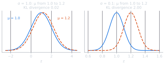
In the one-dimensional example, $F = \mathrm{diag}(1/\sigma^2,\ 2/\sigma^2)$ for the parameters $(\mu, \sigma)$. Each entry is the expected product of two scores. With $s$ standard normal, $\mathrm{E}[s^2] = 1$, $\mathrm{E}[s^4] = 3$ and $\mathrm{E}[s^3] = \mathrm{E}[s] = 0$, so $\mathrm{E}[(s/\sigma)^2] = 1/\sigma^2$, $\mathrm{E}[((s^2 - 1)/\sigma)^2] = (3 - 2 + 1)/\sigma^2 = 2/\sigma^2$, and the cross term $\mathrm{E}[s(s^2 - 1)]/\sigma^2$ vanishes. (The worked example's 100,000 batches estimated the matrix at $\sigma = 0.5$ as $\mathrm{diag}(3.988, 8.006)$ with off-diagonal −0.003, against the exact $\mathrm{diag}(4, 8)$.) For two Gaussians with the same $\sigma$, the divergence is exactly $(\Delta\mu)^2/(2\sigma^2)$, which is the quadratic form $\frac{1}{2}\,\delta\theta^\top F\,\delta\theta$ with $\delta\theta = (\Delta\mu, 0)$; the figure above shows what that $1/\sigma^2$ means. Multiplying the plain log-derivatives by $F^{-1}$ gives
$$\tilde{\nabla}_\mu \log \pi = \sigma s, \qquad \tilde{\nabla}_\sigma \log \pi = \frac{\sigma (s^2 - 1)}{2}.$$
Now both steps are proportional to $\sigma$: the mean moves by a multiple of the current spread, and the spread changes by a fraction of itself. The update is the same whether the distribution is wide or narrow, which is the scale invariance the plain gradient lacked. For the exact gradient of the worked example, $(2, 1)$ at $\mu = 1$, $\sigma = 0.5$, the natural gradient is $F^{-1}(2, 1) = (2\mu\sigma^2,\ \sigma^3) = (0.5, 0.125)$: four times shorter in $\mu$ and eight times shorter in $\sigma$, because at $\sigma = 0.5$ a unit change of either parameter is a large change of the distribution.
The difference decides whether the search converges. nes_worked.py minimizes $z^2$ from $\mu = 1$, $\sigma = 1$ with ten samples per iteration, the rank-based utilities described in the next section, and the same learning rate $\eta = 0.1$ for both methods. The plain update adds $\eta\sum_k u_k s_k/\sigma$ to $\mu$ and $\eta\sum_k u_k(s_k^2 - 1)/\sigma$ to $\sigma$; the natural update adds $\eta\sigma\sum_k u_k s_k$ and $\eta(\sigma/2)\sum_k u_k (s_k^2 - 1)$. In 30 runs, the plain update drove $\sigma$ below zero, an invalid distribution, in 29, after a median of 13 iterations (range 11 to 57); the remaining run ended far from the optimum. The natural update reached $\mu^2 + \sigma^2 \le 10^{-8}$ in all 30 runs, after a median of 212 iterations (IQR 208 to 216), and kept converging linearly.
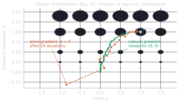
Wierstra et al. (2014, Fig. 2) describe the general effect: directions in which the gradient samples vary a great deal are shrunk, and directions in which they are consistent are boosted.
The canonical NES algorithm estimates $F$ from the same samples as the gradient and solves for the natural gradient. For a full Gaussian in $d$ dimensions, $\theta$ has $d(d+3)/2$ components, so a naive inversion of $F$ costs $O(d^6)$ operations. The later algorithms avoid that entirely, as described below.
Fitness shaping
Raw fitness values make the update sensitive to their scale and to outliers: one lucky sample with an enormous score can dominate the estimate. NES therefore replaces fitness by utilities that depend only on rank (Wierstra et al., 2008). The $k$-th best of $\lambda$ samples receives
$$u_k = \frac{\max\bigl(0,\ \ln(\tfrac{\lambda}{2} + 1) - \ln k\bigr)}{\sum_{j=1}^{\lambda} \max\bigl(0,\ \ln(\tfrac{\lambda}{2} + 1) - \ln j\bigr)} - \frac{1}{\lambda},$$
and the gradient estimate becomes $\sum_k u_k \nabla_\theta \log \pi(\mathbf{z}_k \mid \theta)$ (Wierstra et al., 2014, §3.1). For $\lambda = 10$ the utilities are 0.330, 0.163, 0.066, −0.003, −0.056, and −0.100 for each of the five worst. They sum to zero, which acts as a baseline: samples with negative utility push the distribution away from themselves. Wierstra et al. describe it as the CMA-ES weighting scheme shifted so that the values sum to zero, and like those weights it makes the algorithm invariant to any strictly increasing transformation of the fitness. Wierstra et al. report that the exact shape matters little as long as it is monotone and based on ranks.
xNES and SNES
Exponential NES (xNES; Glasmachers, Schaul, Sun, Wierstra, and Schmidhuber, 2010) makes the natural gradient cheap by computing it in local coordinates in which the current distribution is the standard normal. Write the covariance as $\Sigma = \sigma^2 \mathbf{B}^\top\mathbf{B}$, with a scalar step size $\sigma$ and a shape matrix $\mathbf{B}$ of determinant 1, and sample $\mathbf{z}_k = \boldsymbol{\mu} + \sigma \mathbf{B}^\top \mathbf{s}_k$ with $\mathbf{s}_k \sim \mathcal{N}(\mathbf{0}, \mathbf{I})$. In these coordinates the Fisher matrix of a Gaussian is the identity, so the plain and natural gradients coincide (Wierstra et al., 2014, §3.3.1):
$$\nabla_\delta J = \sum_k u_k \mathbf{s}_k, \qquad \nabla_M J = \sum_k u_k (\mathbf{s}_k \mathbf{s}_k^\top - \mathbf{I}),$$
and the updates are
$$\boldsymbol{\mu} \leftarrow \boldsymbol{\mu} + \eta_\mu \sigma \mathbf{B}^\top \nabla_\delta J, \qquad \sigma \leftarrow \sigma \exp\!\bigl(\tfrac{\eta_\sigma}{2} \nabla_\sigma J\bigr), \qquad \mathbf{B} \leftarrow \mathbf{B} \exp\!\bigl(\tfrac{\eta_B}{2} \nabla_B J\bigr),$$
where $\nabla_\sigma J = \mathrm{tr}(\nabla_M J)/d$ is the part of the covariance gradient that changes the overall scale and $\nabla_B J = \nabla_M J - \nabla_\sigma J\, \mathbf{I}$ is the rest. The matrix exponential keeps the covariance positive definite, and separating $\sigma$ from $\mathbf{B}$ allows independent learning rates for scale and shape. The one-dimensional formulas above are this update with $\mathbf{B} = 1$, apart from the exponential. The defaults are $\lambda = 4 + \lfloor 3 \ln d \rfloor$, the same as CMA-ES, $\eta_\mu = 1$, and $\eta_\sigma = \eta_B = (9 + 3\ln d)/(5d\sqrt{d})$ (Wierstra et al., 2014, Table 1). Each update still costs $O(d^3)$.
Separable NES (SNES; Schaul, Glasmachers, and Schmidhuber, 2011) restricts the covariance to a diagonal, with one step size $\sigma_i$ per coordinate:
$$\boldsymbol{\mu} \leftarrow \boldsymbol{\mu} + \eta_\mu\, \boldsymbol{\sigma} \odot \sum_k u_k \mathbf{s}_k, \qquad \boldsymbol{\sigma} \leftarrow \boldsymbol{\sigma} \odot \exp\!\Bigl(\tfrac{\eta_\sigma}{2} \sum_k u_k (\mathbf{s}_k \odot \mathbf{s}_k - \mathbf{1})\Bigr),$$
where $\odot$ is the elementwise product. The cost is linear in $d$, which makes SNES usable for neural networks with many weights, and with only $d$ variance parameters to learn, the learning rate can be larger, $\eta_\sigma = (3 + \ln d)/(5\sqrt{d})$ (Wierstra et al., 2014, §5.1). The price is that SNES cannot learn correlations between variables.
The link to CMA-ES
The xNES covariance update, expanded to first order, is
$$\Sigma \leftarrow (1 - U \eta_\Sigma)\, \Sigma + \eta_\Sigma \sum_k u_k (\mathbf{z}_k - \boldsymbol{\mu})(\mathbf{z}_k - \boldsymbol{\mu})^\top, \qquad U = \sum_k u_k,$$
which has the form of the rank-μ update of CMA-ES, with utilities in place of recombination weights (Glasmachers et al., 2010; Wierstra et al., 2014, §4). Akimoto, Nagata, Ono, and Kobayashi (2010) showed the connection from the other side: the CMA-ES updates of the mean and covariance, without evolution paths, approximately follow the natural gradient of expected fitness, and Akimoto et al. (2012) developed the information-geometric analysis further. The two families differ in what the derivation does not cover. CMA-ES has evolution paths, so its state is not fully described by its current distribution; it updates the covariance additively where xNES updates it multiplicatively; and both use different learning rates for the mean and the covariance, so that, strictly, neither follows the natural gradient (Wierstra et al., 2014, §4). The step-size control and the rank-one update of CMA-ES, which rely on evolution paths, are not covered by this derivation.
On the BBOB benchmark of 24 noiseless and 30 noisy functions, Wierstra et al. (2014, §5.2) found xNES among the best algorithms benchmarked in 2009, provided the budget exceeds about $100d$ evaluations. With its default settings it was weak on highly multimodal functions such as Rastrigin's, where they suggest larger populations and restart strategies.
Measured on benchmark functions
The script tools/experiments/evolution/nes.py in the site repository implements SNES with the defaults above and compares it with the CMA-ES runs of cmaes.py on the same functions, starts and seeds: $d = 10$, $\boldsymbol{\mu}_0$ uniform in $[-2, 2]^{10}$, $\sigma_0 = 1.2$, budget $10^5$ evaluations, target $f \le 10^{-8}$, seeds 0 to 29. Both algorithms use $\lambda = 10$.
| Function ($d = 10$) | SNES, evaluations to $10^{-8}$ | CMA-ES (from the CMA-ES article) |
|---|---|---|
| Sphere | 1,900 [1,863, 1,926], 30/30 | 1,344 [1,314, 1,379], 30/30 |
| Ellipsoid, axis-parallel, condition $10^6$ | 2,752 [2,706, 2,790], 30/30 | 5,628 [5,469, 5,694], 30/30 |
| Same ellipsoid, rotated | 0/30 within $10^5$ | 5,519 [5,416, 5,746], 30/30 |
Medians with interquartile ranges. On the axis-parallel ellipsoid, SNES is twice as fast as CMA-ES. The likely reason is that it needs to learn only ten variances, with a learning rate ($\eta_\sigma = 0.335$ for $d = 10$) far larger than the rates CMA-ES uses for its 55 covariance entries ($c_1 = 0.015$, $c_\mu = 0.024$). Rotate the same ellipsoid and SNES no longer reaches the target; after $10^5$ evaluations the median $f(\boldsymbol{\mu})$ is 230. A diagonal covariance cannot align with axes that are not the coordinate axes. This is the trade-off a separable method makes, in exchange for linear cost.
OpenAI's evolution strategy
Salimans et al. (2017) took the NES idea in the opposite direction from xNES: they removed nearly everything except the search gradient for the mean. The search distribution is an isotropic Gaussian with a fixed standard deviation $\sigma$ around the parameter vector $\theta$ of a neural network policy, so the objective becomes the Gaussian-blurred return $\mathrm{E}_{\boldsymbol{\epsilon} \sim \mathcal{N}(\mathbf{0}, \mathbf{I})} F(\theta + \sigma\boldsymbol{\epsilon})$, and its gradient is
$$\nabla_\theta\, \mathrm{E}_{\boldsymbol{\epsilon}}\, F(\theta + \sigma\boldsymbol{\epsilon}) = \frac{1}{\sigma}\, \mathrm{E}_{\boldsymbol{\epsilon}}\bigl[F(\theta + \sigma\boldsymbol{\epsilon})\, \boldsymbol{\epsilon}\bigr].$$
Each iteration samples $n$ perturbations, runs one episode with each perturbed policy to get returns $F_i$, and updates $\theta \leftarrow \theta + \frac{\alpha}{n\sigma} \sum_i F_i \boldsymbol{\epsilon}_i$. With $\sigma$ fixed and isotropic, the Fisher matrix for the mean is a multiple of the identity, so the natural and plain gradients point the same way, and nothing else is adapted. The authors note that the estimator is also known as simultaneous perturbation stochastic approximation, parameter-exploring policy gradients, or zero-order gradient estimation. They added three standard techniques: antithetic (mirrored) sampling, which evaluates each $\boldsymbol{\epsilon}$ together with $-\boldsymbol{\epsilon}$ to reduce variance; fitness shaping by a rank transformation of the returns, which they found reduced the influence of outliers and the tendency to fall into local optima early; and weight decay. Unlike NES, they saw no benefit from adapting $\sigma$.
Why antithetic sampling helps. Expand the return around $\theta$: $F(\theta + \sigma\boldsymbol{\epsilon}) = F(\theta) + \sigma\,\mathbf{g}^\top\boldsymbol{\epsilon} + \frac{\sigma^2}{2}\boldsymbol{\epsilon}^\top \mathbf{H}\boldsymbol{\epsilon} + \dots$, with gradient $\mathbf{g}$ and Hessian $\mathbf{H}$. A single sample's contribution $F(\theta + \sigma\boldsymbol{\epsilon})\,\boldsymbol{\epsilon}/\sigma$ therefore contains the term $F(\theta)\,\boldsymbol{\epsilon}/\sigma$, which has mean zero but is enormous when $F(\theta)$ is large compared with $\sigma\lVert\mathbf{g}\rVert$; it is pure noise. For a mirrored pair, the even terms cancel, $$\frac{F(\theta + \sigma\boldsymbol{\epsilon}) - F(\theta - \sigma\boldsymbol{\epsilon})}{2\sigma}\,\boldsymbol{\epsilon} = (\mathbf{g}^\top\boldsymbol{\epsilon})\,\boldsymbol{\epsilon} + O(\sigma^2),$$ so both the constant $F(\theta)$ and the curvature term disappear, exactly so for a quadratic $F$. What remains, $(\mathbf{g}^\top\boldsymbol{\epsilon})\boldsymbol{\epsilon}$, is an unbiased estimate of $\mathbf{g}$ whose mean squared error is $(d + 1)\lVert\mathbf{g}\rVert^2$, since $\mathrm{E}[(\mathbf{g}^\top\boldsymbol{\epsilon})^2\lVert\boldsymbol{\epsilon}\rVert^2] = (d + 2)\lVert\mathbf{g}\rVert^2$. Antithetic sampling acts as a baseline that needs no knowledge of $F(\theta)$.
nes_worked.py measures the effect for $F(\theta) = -\lVert\theta\rVert^2$ in $d = 10$ dimensions at a point with $\lVert\theta\rVert = 1$, so $F(\theta) = -1$ and $\lVert\mathbf{g}\rVert = 2$, with $\sigma = 0.1$ and 20 evaluations per estimate (100,000 estimates each):
| Estimator, 20 evaluations | Mean squared error | Mean cosine with the true gradient |
|---|---|---|
| Plain, 20 independent samples | 65.3 | 0.23 |
| Plain with $F(\theta)$ subtracted (needs $F(\theta)$) | 3.05 | 0.78 |
| Antithetic, 10 mirrored pairs | 4.40 | 0.72 |
The plain estimator's error is dominated by the $F(\theta)\boldsymbol{\epsilon}/\sigma$ term, which alone contributes $d\,F(\theta)^2/\sigma^2/20 = 50$; with it, the estimate's cosine with the true direction averages only 0.23. The antithetic estimator's error matches the formula, $(d + 1)\lVert\mathbf{g}\rVert^2/10 = 4.4$, fifteen times lower. Subtracting a known $F(\theta)$ is slightly better still, because it spends all 20 evaluations on different directions, but it requires an extra evaluation at $\theta$ in every iteration, and in reinforcement learning, where returns are noisy, a single evaluation of $F(\theta)$ is itself unreliable. The rank transformation of the returns has a similar centering effect, since ranks mapped to $[-0.5, 0.5]$ sum to zero.
Shared random seeds. The contribution that made the method scale was in communication. Each worker evaluates one perturbation and must learn every other worker's perturbation to compute the update. Sending million-dimensional noise vectors would be as expensive as sending gradients. Instead, the workers agree on random seeds before training, so each can regenerate every $\boldsymbol{\epsilon}_j$ itself, and only the scalar returns need to be exchanged. In practice each worker creates a large block of Gaussian noise at the start of training and forms each perturbation from a randomly indexed part of it (Salimans et al., 2017, §2.1). The same design is discussed as a case of master-slave parallel evaluation.
What was reported. The results, stated as the paper states them:
- On the MuJoCo 3D humanoid walking task, the median time over 7 repeats to reach a score of 6,000 fell from 657 minutes on 18 CPU cores to 10 minutes on 1,440, a linear speedup in the number of cores.
- On 51 Atari games, trained for 1 billion frames each on 720 CPUs, about one hour per game, ES did better than the published 1-day results of A3C on 23 games and worse on 28. The authors estimate that the two use about the same amount of neural network computation, because ES needs no backpropagation and no value function, although ES needed 3 to 10 times as much data to match A3C's final performance on most games.
- On MuJoCo tasks, ES needed less than 10 times the environment interaction of TRPO, a tuned policy gradient method, to reach TRPO's performance after 5 million steps on the hard tasks (Hopper and Walker2d), and up to 3 times less on simple ones, measured on mean curves over 6 seeds.
- Reliability on Atari depended on virtual batch normalization in the network, and some MuJoCo tasks needed discretized actions to encourage exploration.
The authors also argue that, because ES perturbs parameters rather than actions, the variance of its gradient estimate does not grow with the length of an episode, while that of a policy gradient estimate grows nearly linearly with it; ES is therefore attractive for long episodes with delayed rewards, and in their Pong experiment it was insensitive to the frame-skip setting (Salimans et al., 2017, §3.1, §4.4).
What the follow-ups clarified
Salimans et al. (2017, §3.2) observed that their gradient estimate is a finite-difference derivative in a random direction. Later work took up two questions: whether an algorithm that does not estimate a gradient at all could also work at that scale, and how good the estimate really is.
A gradient-free genetic algorithm. Such, Madhavan, Conti, Lehman, Stanley, and Clune (2017) evolved networks with over four million parameters using a plain genetic algorithm: truncation selection, parents chosen uniformly from the top $T$, Gaussian mutation, one elite, and no crossover. On 13 Atari games it was roughly competitive with DQN, A3C and ES, each method doing best on different games. It beat random search on every game, but random search alone beat DQN on 3 games, ES on 3, and A3C on 6, a reminder that baselines are needed to tell what the optimizer contributes. They stored each network as the list of random seeds that generated its mutations, a compression of up to 10,000-fold. The fixed-topology neuroevolution article describes this work in more detail.
How good the gradient is. Zhang, Clune, and Stanley (2017) compared the ES update with the true gradient on MNIST, where the gradient is available. With 10,000 perturbations per step, the correlation between the ES gradient and the stochastic gradient descent gradient averaged only 3.9%, yet after 2,000 iterations ES reached a mean validation accuracy of 96.99% over 5 runs, against 98.69% for SGD. Using an SGD-based proxy, they estimated that a correlation of about 20% would bring ES close to SGD's accuracy, and with further changes they reached 99% accuracy with ES. They did not suggest using ES for supervised learning, where exact gradients are cheap.
What the blurred objective rewards. Lehman, Chen, Clune, and Stanley (2018) showed that this ES is more than a finite-difference approximator. Because it maximizes the average return of the perturbed population, not the return of $\theta$ itself, it is drawn toward regions where the return is robust to perturbation. On their two-dimensional test functions, ES with a large $\sigma$ could not follow a path that narrows toward higher fitness, but could cross a gap that stopped finite-difference gradient descent. On the humanoid task, policies trained by ES lost much less performance under random parameter perturbation than policies of similar return trained by the genetic algorithm of Such et al. or by TRPO. With small $\sigma$ the behavior approaches that of finite differences. Whether robustness is desirable depends on the task.
A small experiment
nes.py also runs the OpenAI-style update (antithetic pairs, ranks mapped linearly to $[-0.5, 0.5]$, fixed $\sigma$ and $\alpha$, plain gradient steps) on the 10-dimensional sphere with 5 pairs per iteration. With $\sigma = 0.1$ and $\alpha = 0.01$, the median $f(\theta)$ over 30 seeds is 0.93 after 1,000 evaluations, $1.1 \times 10^{-4}$ after 10,000, and $8.8 \times 10^{-5}$ after 100,000. With $\sigma = 0.01$ and $\alpha = 0.001$ the medians are $1.6 \times 10^{-3}$, $1.6 \times 10^{-3}$ and $1.1 \times 10^{-3}$ after 10,000, 50,000 and 100,000 evaluations. The method nearly stalls: the level it settles toward is set by $\sigma$ and $\alpha$, and a larger budget improves it only slowly. A likely reason is that the rank transformation keeps the length of the update roughly constant even near the optimum, so with fixed $\alpha$ and $\sigma$ the iterates keep moving at that scale. SNES, which adapts $\sigma$, reaches $10^{-8}$ in a median of 1,900 evaluations. For policy search this is not a defect, since precise convergence is rarely the goal, but it rules the method out for precise numerical optimization.
The script then trains a linear threshold policy (5 parameters) for a cart-pole balancing task of the kind introduced by Barto, Sutton, and Anderson (1983), with the constants listed in the script. Fitness is the number of steps the pole stays up in one episode from a random start, capped at 500, and a run counts as solved when its current policy balances for 500 steps from each of 20 fixed test starts. Over 30 seeds, counting training episodes until solved:
| Method | Solved | Training episodes, median [IQR] | Range |
|---|---|---|---|
| OpenAI-style ES, 10 pairs, $\sigma = 0.1$, $\alpha = 0.05$ | 30/30 | 260 [185, 380] | 100 to 460 |
| SNES, $\lambda = 8$, $\sigma_0 = 0.1$ | 30/30 | 80 [72, 118] | 24 to 312 |
| Random search, $\theta \sim \mathcal{N}(\mathbf{0}, \mathbf{I})$ | 30/30 | 304 [122, 754] | 15 to 2,023 |
Random search does nearly as well as the OpenAI-style ES at the median, although with a much wider spread. A five-parameter linear controller for cart-pole is easy enough that a few hundred random draws usually include a good policy. The experiment demonstrates the mechanics, not an advantage, and it repeats on a small scale the point of Such et al.: without a random-search baseline, an evolutionary method's success on a task is hard to interpret.
Where this leaves evolution strategies
The natural gradient view gives evolution strategies a derivation that machine learning researchers recognize: estimate a gradient of expected fitness with respect to the parameters of the search distribution, precondition it by the geometry of that distribution, and step. It explains much of CMA-ES and none of its evolution paths. The reinforcement learning work showed a different strength, scale: an algorithm whose workers exchange one number each can use a thousand processors with very little communication. Its weaknesses are those of its simplicity: no adaptation of $\sigma$, a gradient estimate that, like other randomized finite-difference schemes, can need a number of steps that grows with the dimension, although Salimans et al. (2017, §3.2) argue that the problem's intrinsic dimension matters more than the number of parameters, and, on easy problems, little to distinguish it from random search. Evolving the network structure as well as the weights is a different line of work, taken up in NEAT and the rest of neuroevolution.
References
- Akimoto, Y., Nagata, Y., Ono, I., and Kobayashi, S. (2010). Bidirectional relation between CMA evolution strategies and natural evolution strategies. In Parallel Problem Solving from Nature, PPSN XI, Lecture Notes in Computer Science 6238, 154–163. Springer.
- Akimoto, Y., Nagata, Y., Ono, I., and Kobayashi, S. (2012). Theoretical foundation for CMA-ES from information geometry perspective. Algorithmica, 64(4), 698–716.
- Amari, S. (1998). Natural gradient works efficiently in learning. Neural Computation, 10(2), 251–276.
- Barto, A. G., Sutton, R. S., and Anderson, C. W. (1983). Neuronlike adaptive elements that can solve difficult learning control problems. IEEE Transactions on Systems, Man, and Cybernetics, SMC-13(5), 834–846.
- Glasmachers, T., Schaul, T., Sun, Y., Wierstra, D., and Schmidhuber, J. (2010). Exponential natural evolution strategies. In Proceedings of the 12th Annual Conference on Genetic and Evolutionary Computation (GECCO 2010), 393–400.
- Lehman, J., Chen, J., Clune, J., and Stanley, K. O. (2018). ES is more than just a traditional finite-difference approximator. In Proceedings of the Genetic and Evolutionary Computation Conference (GECCO 2018), 450–457.
- Salimans, T., Ho, J., Chen, X., Sidor, S., and Sutskever, I. (2017). Evolution strategies as a scalable alternative to reinforcement learning. arXiv:1703.03864.
- Schaul, T., Glasmachers, T., and Schmidhuber, J. (2011). High dimensions and heavy tails for natural evolution strategies. In Proceedings of the 13th Annual Conference on Genetic and Evolutionary Computation (GECCO 2011), 845–852.
- Such, F. P., Madhavan, V., Conti, E., Lehman, J., Stanley, K. O., and Clune, J. (2017). Deep neuroevolution: genetic algorithms are a competitive alternative for training deep neural networks for reinforcement learning. arXiv:1712.06567.
- Wierstra, D., Schaul, T., Glasmachers, T., Sun, Y., Peters, J., and Schmidhuber, J. (2014). Natural evolution strategies. Journal of Machine Learning Research, 15, 949–980.
- Wierstra, D., Schaul, T., Peters, J., and Schmidhuber, J. (2008). Natural evolution strategies. In Proceedings of the 2008 IEEE Congress on Evolutionary Computation, 3381–3387.
- Williams, R. J. (1992). Simple statistical gradient-following algorithms for connectionist reinforcement learning. Machine Learning, 8(3–4), 229–256.
- Zhang, X., Clune, J., and Stanley, K. O. (2017). On the relationship between the OpenAI evolution strategy and stochastic gradient descent. arXiv:1712.06564.