Consider minimizing $f(\mathbf{x}) = \sum_{i=1}^{10} 10^{6(i-1)/9} x_i^2$, an ellipsoid whose axes differ in curvature by a factor of a million. A search that mutates every coordinate with the same step size has to choose between steps small enough for the steepest axis and steps large enough to make progress along the flattest one. The 1/5 success rule and self-adaptation can tune one step size, or one per coordinate, but neither helps much when the ellipsoid is rotated so that its axes no longer line up with the coordinates. What the search needs is a mutation distribution shaped like the function's contour lines.
The covariance matrix adaptation evolution strategy (CMA-ES) learns that shape. It samples candidate solutions from a multivariate normal distribution and adapts the distribution's mean, its overall step size, and its full covariance matrix from the ranking of the samples. On the ellipsoid above, the implementation described below needs a median of 5,628 evaluations to reach $f \le 10^{-8}$, and 5,519 when the same ellipsoid is rotated at random. The algorithm was introduced by Hansen and Ostermeier (1996, 2001); the rank-$\mu$ update was added by Hansen, Müller, and Koumoutsakos (2003). This article follows the formulation and default parameters of Hansen's tutorial (Hansen, 2016), whose Appendix A is the reference specification. The broader family is introduced in evolution strategies, and its history in the history of evolutionary computation.
Sampling
Each generation $g$ draws $\lambda$ new points:
$$\mathbf{x}_k = \mathbf{m} + \sigma \mathbf{y}_k, \qquad \mathbf{y}_k \sim \mathcal{N}(\mathbf{0}, \mathbf{C}), \qquad k = 1, \dots, \lambda.$$
Here $\mathbf{m} \in \mathbb{R}^n$ is the mean of the search distribution, the current best guess at the optimum; $\sigma > 0$ is the overall step size; and $\mathbf{C}$ is a symmetric positive definite $n \times n$ covariance matrix, which sets the distribution's shape. The sample is $\mathcal{N}(\mathbf{m}, \sigma^2 \mathbf{C})$. To draw it, CMA-ES uses the eigendecomposition $\mathbf{C} = \mathbf{B}\mathbf{D}^2\mathbf{B}^\top$, where the columns of the orthogonal matrix $\mathbf{B}$ are the eigenvectors of $\mathbf{C}$ and the diagonal matrix $\mathbf{D}$ holds the square roots of its eigenvalues. A vector $\mathbf{z} \sim \mathcal{N}(\mathbf{0}, \mathbf{I})$ of independent standard normal numbers becomes $\mathbf{y} = \mathbf{B}\mathbf{D}\mathbf{z}$: $\mathbf{D}$ stretches the sphere along the coordinate axes, and $\mathbf{B}$ rotates the result. The surfaces of equal density are ellipsoids whose principal axes are the eigenvectors (Hansen, 2016, §0.2).
Selection and weighted recombination
The $\lambda$ points are ranked by $f$, and $\mathbf{x}_{i:\lambda}$ denotes the $i$-th best. The new mean is a weighted average of the best $\mu$:
$$\mathbf{m} \leftarrow \sum_{i=1}^{\mu} w_i \mathbf{x}_{i:\lambda}, \qquad w_1 \ge w_2 \ge \dots \ge w_\mu > 0, \qquad \sum_{i=1}^{\mu} w_i = 1.$$
This is truncation selection followed by weighted intermediate recombination, the $(\mu/\mu_W, \lambda)$ scheme of comma selection: the parents are discarded every generation. The defaults set $\mu = \lfloor \lambda/2 \rfloor$ and $w_i \propto \ln\frac{\lambda+1}{2} - \ln i$. For $n = 10$, $\lambda = 10$ and $\mu = 5$, the raw values $\ln 5.5 - \ln i$ are 1.705, 1.012, 0.606, 0.318 and 0.095, which normalize to
$$w = (0.456,\ 0.271,\ 0.162,\ 0.085,\ 0.026).$$
The quantity that governs how much information the average carries is the variance effective selection mass,
$$\mu_{\text{eff}} = \frac{1}{\sum_{i=1}^{\mu} w_i^2},$$
which lies between 1 and $\mu$ and equals $\mu$ for equal weights. Averaging $\mu$ independent samples with these weights reduces their variance by a factor of $\mu_{\text{eff}}$ (Hansen, 2016, §2). For the weights above, $\mu_{\text{eff}} = 3.167$.
The reason is one line of algebra. If selection carried no information, the selected steps $\mathbf{y}_{i:\lambda}$ would be independent draws from $\mathcal{N}(\mathbf{0}, \mathbf{C})$, and the covariance of their weighted sum would be
$$\mathrm{Cov}\Bigl(\sum_{i=1}^{\mu} w_i \mathbf{y}_{i:\lambda}\Bigr) = \sum_{i=1}^{\mu} w_i^2\, \mathbf{C} = \frac{\mathbf{C}}{\mu_{\text{eff}}}.$$
So $\sqrt{\mu_{\text{eff}}}$ times the weighted mean step has the same distribution as a single step. The normalizing constants of both evolution paths below use exactly this factor. With equal weights the average of $\mu$ steps would have variance $\mathbf{C}/\mu$; the decreasing weights trade some of that averaging for a stronger emphasis on the best samples, and $\mu_{\text{eff}}$ is the number of equally weighted samples that would give the same variance.
Only the ranking of the $\lambda$ values enters the algorithm, never the values themselves. That is the source of the first of its invariances, discussed below.
Step-size control: the evolution path $p_\sigma$
Covariance adaptation alone cannot set the overall step length well, for two reasons Hansen (2016, §4) gives. The optimal step size depends on $\mu_{\text{eff}}$ in a way the covariance update does not capture, and the covariance learning rates are too small to change the scale as fast as progress on a simple function such as the sphere requires. CMA-ES therefore controls $\sigma$ separately, by cumulative step-size adaptation (CSA), which looks at the path the mean has taken over recent generations.
The reasoning is geometric. If consecutive steps of the mean point in similar directions, the same distance could have been covered with fewer, longer steps, so $\sigma$ should grow. If they cancel each other out, the search is circling the optimum and $\sigma$ should shrink. If they are uncorrelated, as consecutive steps are under random selection, $\sigma$ is about right. CSA accumulates the steps in an evolution path with exponential smoothing,
$$\mathbf{p}_\sigma \leftarrow (1 - c_\sigma)\mathbf{p}_\sigma + \sqrt{c_\sigma(2 - c_\sigma)\mu_{\text{eff}}}\; \mathbf{C}^{-1/2} \langle \mathbf{y} \rangle_w, \qquad \langle \mathbf{y} \rangle_w = \sum_{i=1}^{\mu} w_i \mathbf{y}_{i:\lambda},$$
where $\langle \mathbf{y} \rangle_w = (\mathbf{m}_{\text{new}} - \mathbf{m}_{\text{old}})/\sigma$ is the step of the mean without the step size, and $\mathbf{C}^{-1/2} = \mathbf{B}\mathbf{D}^{-1}\mathbf{B}^\top$. The factor $\mathbf{C}^{-1/2}$ removes the shape of the distribution, so that the path's expected length does not depend on its direction. The constant $\sqrt{c_\sigma(2-c_\sigma)\mu_{\text{eff}}}$ is chosen so that, under random selection, $\mathbf{p}_\sigma \sim \mathcal{N}(\mathbf{0}, \mathbf{I})$. The step size is then compared with that reference:
$$\sigma \leftarrow \sigma \exp\!\left(\frac{c_\sigma}{d_\sigma}\left(\frac{\lVert \mathbf{p}_\sigma \rVert}{\mathrm{E}\lVert \mathcal{N}(\mathbf{0}, \mathbf{I}) \rVert} - 1\right)\right),$$
with $\mathrm{E}\lVert \mathcal{N}(\mathbf{0}, \mathbf{I}) \rVert = \sqrt{2}\,\Gamma(\frac{n+1}{2})/\Gamma(\frac{n}{2}) \approx \sqrt{n}\,(1 - \frac{1}{4n} + \frac{1}{21n^2})$, which is 3.084 for $n = 10$. A path longer than expected increases $\sigma$, a shorter one decreases it, and the damping $d_\sigma \approx 1$ limits the change per generation. Under random selection the update leaves $\ln \sigma$ unbiased, which guards against both divergence and premature convergence when selection carries little information (Hansen, 2016, §5).
Where the normalizing constant comes from. Under random selection, $\mathbf{C}^{-1/2}\langle \mathbf{y} \rangle_w$ is normal with covariance $\mathbf{I}/\mu_{\text{eff}}$, by the variance calculation above, and it is independent from one generation to the next. Write the update as $\mathbf{p} \leftarrow (1 - c)\mathbf{p} + a\,\boldsymbol{\xi}$ with $\boldsymbol{\xi} \sim \mathcal{N}(\mathbf{0}, \mathbf{I}/\mu_{\text{eff}})$. If $\mathbf{p}$ has covariance $v\mathbf{I}$, the new path has covariance $\bigl((1 - c)^2 v + a^2/\mu_{\text{eff}}\bigr)\mathbf{I}$. The stationary value solves $v = (1 - c)^2 v + a^2/\mu_{\text{eff}}$, so $$v = \frac{a^2}{\mu_{\text{eff}}\,\bigl(1 - (1 - c)^2\bigr)} = \frac{a^2}{\mu_{\text{eff}}\, c\,(2 - c)},$$ and $v = 1$ exactly when $a = \sqrt{c(2 - c)\mu_{\text{eff}}}$. The path then has the distribution $\mathcal{N}(\mathbf{0}, \mathbf{I})$ whenever selection is random, and its length can be compared with $\mathrm{E}\lVert \mathcal{N}(\mathbf{0}, \mathbf{I}) \rVert$ without any further calibration. The same argument fixes the constant $\sqrt{c_c(2 - c_c)\mu_{\text{eff}}}$ of the second path below, which has covariance $\mathbf{C}$ under random selection. The factor $\sqrt{1 - (1 - c_\sigma)^{2g}}$ in the indicator $h_\sigma$ below is the same calculation stopped after $g$ generations, starting from $\mathbf{p}_\sigma = \mathbf{0}$.
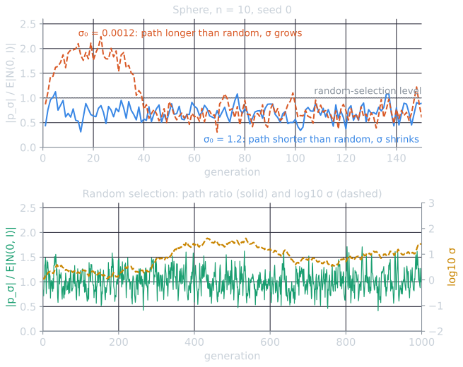
The script tools/experiments/evolution/cmaes_components.py measured these traces. In the sphere run with $\sigma_0 = 1.2$, the ratio $\lVert \mathbf{p}_\sigma \rVert / \mathrm{E}\lVert \mathcal{N}(\mathbf{0}, \mathbf{I}) \rVert$ averaged 0.701 over generations 21 to 150, and $\sigma$ fell from 1.2 to 0.047 after 50 generations and $6.5 \times 10^{-5}$ after 150, in step with the distance to the optimum. With $\sigma_0 = 0.0012$ the ratio passed 1.4 in the third generation and reached 1.9 by the tenth, $\sigma$ grew tenfold by generation 16 and peaked at 0.56 in generation 39. Under random selection, over generations 50 to 1,000, the ratio averaged 1.009, with 90% of values between 0.64 and 1.39. "Unbiased" does not mean "stationary": without selection $\log_{10}\sigma$ wandered, from 0.08 at the start to 1.50 after 500 generations and 1.41 after 1,000. The rule has no preferred step size of its own; it only reacts to what selection does to the path.
CSA is the main difference from the step-size rules in the earlier articles of this topic. The 1/5 rule measures success rates, and self-adaptation mutates step sizes along with the individuals that carry them. CSA uses neither: given the sampled points, the new step size is a deterministic function of the selected steps. Hansen and Ostermeier (2001) present derandomization, adapting the distribution so as to favor previously selected mutation steps, and cumulation, using an evolution path rather than single steps, as the two ideas behind CMA.
Covariance matrix adaptation
The rank-μ update
Suppose $\sigma = 1$ for the moment. A natural idea is to re-estimate the covariance from the selected points. Estimation of distribution algorithms such as EMNA do this with the variance of the selected points around their own mean. CMA-ES instead measures the selected steps from the old mean:
$$\mathbf{C}_\mu = \sum_{i=1}^{\mu} w_i\, \mathbf{y}_{i:\lambda} \mathbf{y}_{i:\lambda}^\top, \qquad \mathbf{y}_{i:\lambda} = \frac{\mathbf{x}_{i:\lambda} - \mathbf{m}_{\text{old}}}{\sigma}.$$
The difference matters. On a linear function, the variance of the selected points around their own mean shrinks geometrically in the direction of improvement, which makes a search built on it highly susceptible to premature convergence; the variance of the selected steps grows in that direction (Hansen, 2016, §3.1, Fig. 3). Sampling from $\mathbf{C}_\mu$ tends to reproduce the steps that were selected.
A single generation of a small population cannot estimate a full covariance matrix reliably; Hansen (2016, §3.1) reports that a condition number below ten on the sphere needs $\mu_{\text{eff}} \approx 10n$. The rank-μ update therefore blends each generation's estimate into the old matrix with a small learning rate $c_\mu$:
$$\mathbf{C} \leftarrow (1 - c_\mu)\mathbf{C} + c_\mu \sum_{i=1}^{\mu} w_i\, \mathbf{y}_{i:\lambda} \mathbf{y}_{i:\lambda}^\top.$$
Information older than about $1/c_\mu$ generations has decayed to about 37% of its original weight. The name refers to the rank of the added sum, $\min(\mu, n)$.
The rank-one update and the evolution path $p_c$
The outer product $\mathbf{y}\mathbf{y}^\top$ equals $(-\mathbf{y})(-\mathbf{y})^\top$, so the rank-μ update discards the sign of each step: whether the search went up or down a valley makes no difference to it. A second evolution path restores that information by summing successive steps of the mean,
$$\mathbf{p}_c \leftarrow (1 - c_c)\mathbf{p}_c + h_\sigma \sqrt{c_c(2-c_c)\mu_{\text{eff}}}\; \langle \mathbf{y} \rangle_w,$$
and the rank-one update adds $c_1 \mathbf{p}_c \mathbf{p}_c^\top$ to the covariance matrix. If the mean keeps moving in the same direction, the steps add up, $\mathbf{p}_c$ grows by a factor of up to about $1/\sqrt{c_c}$, and the distribution stretches along that direction faster than the learning rate alone would allow. With $1/c_c$ between $\sqrt{n}$ and $n/2$, the number of evaluations needed to learn a single long axis becomes $O(n)$ despite a learning rate $c_1 \approx 2/n^2$ (Hansen, 2016, §3.3.2). Unlike $\mathbf{p}_\sigma$, this path is not normalized by $\mathbf{C}^{-1/2}$, because it is meant to carry the shape.
The indicator $h_\sigma$ is 1 unless $\lVert \mathbf{p}_\sigma \rVert$ is unusually large, specifically unless $\lVert \mathbf{p}_\sigma \rVert / \sqrt{1 - (1 - c_\sigma)^{2g}} \ge (1.4 + \frac{2}{n+1})\, \mathrm{E}\lVert \mathcal{N}(\mathbf{0}, \mathbf{I}) \rVert$ after $g$ generations. A long $\mathbf{p}_\sigma$ means the step size is far too small, for instance at the start of a run on a nearly linear slope; stalling $\mathbf{p}_c$ then prevents the covariance matrix from growing too fast along that slope.
The combined update
The full update combines both terms (Hansen, 2016, eq. 47, here with positive weights only):
$$\mathbf{C} \leftarrow \bigl(1 + c_1\delta(h_\sigma) - c_1 - c_\mu\bigr)\mathbf{C} + \underbrace{c_1 \mathbf{p}_c \mathbf{p}_c^\top}_{\text{rank one}} + \underbrace{c_\mu \sum_{i=1}^{\mu} w_i\, \mathbf{y}_{i:\lambda}\mathbf{y}_{i:\lambda}^\top}_{\text{rank }\mu},$$
where $\delta(h_\sigma) = (1 - h_\sigma)c_c(2 - c_c)$ makes up for the variance lost when $h_\sigma = 0$. The rank-μ term uses the whole population efficiently and matters most with large $\lambda$; the rank-one term exploits correlations between generations and matters most with small $\lambda$ (Hansen, 2016, §3.4).
One generation, in order: sample $\lambda$ points; rank them; move the mean; update $\mathbf{p}_\sigma$ using $\mathbf{C}^{-1/2}$ from before the update; update $\sigma$; update $\mathbf{p}_c$; update $\mathbf{C}$; recompute its eigendecomposition.
Default parameters
Only the initial mean and step size depend on the problem. Hansen (2016, App. A, fn. 1) suggests drawing the initial mean uniformly from the search interval $[a, b]^n$ when one is known, and setting $\sigma = 0.3(b - a)$. Everything else follows from $n$ (Hansen, 2016, Table 1):
| Parameter | Default | $n = 10$ |
|---|---|---|
| Population size $\lambda$ | $4 + \lfloor 3 \ln n \rfloor$ | 10 |
| Parents $\mu$ | $\lfloor \lambda/2 \rfloor$ | 5 |
| Weights $w_i$ | $\propto \ln\frac{\lambda+1}{2} - \ln i$ | $\mu_{\text{eff}} = 3.167$ |
| Mean learning rate $c_m$ | 1 | 1 |
| $c_\sigma$ | $\frac{\mu_{\text{eff}} + 2}{n + \mu_{\text{eff}} + 5}$ | 0.2844 |
| $d_\sigma$ | $1 + 2\max\bigl(0, \sqrt{\frac{\mu_{\text{eff}} - 1}{n+1}} - 1\bigr) + c_\sigma$ | 1.2844 |
| $c_c$ | $\frac{4 + \mu_{\text{eff}}/n}{n + 4 + 2\mu_{\text{eff}}/n}$ | 0.2950 |
| $c_1$ | $\frac{2}{(n + 1.3)^2 + \mu_{\text{eff}}}$ | 0.01528 |
| $c_\mu$ | $\min\Bigl(1 - c_1,\ \frac{2(\mu_{\text{eff}} - 2 + 1/\mu_{\text{eff}} + 1/4)}{(n+2)^2 + \mu_{\text{eff}}}\Bigr)$ | 0.02355 |
The population grows only logarithmically: $\lambda$ is 6 for $n = 2$ and 17 for $n = 100$. The learning rates for $\mathbf{C}$ shrink roughly as $1/n^2$, reflecting the $n(n+1)/2$ parameters of the covariance matrix. Hansen does not recommend changing these settings apart from increasing $\lambda$, which tends to make the search more global at some cost in speed, and possibly lowering the covariance learning rates on noisy functions.
Since 2016 the tutorial's default also gives the worse half of the population negative weights in the covariance update, an idea known as active CMA (Jastrebski and Arnold, 2006), which actively shrinks the variance in directions that produced bad steps. The weights are bounded so that $\mathbf{C}$ stays positive definite. The implementation below omits this, as Hansen's minimal reference implementation purecma does, and uses only the $\mu$ positive weights.
One generation by hand
All of the updates above can be followed with numbers in two dimensions. Take the ellipse
$$f(\mathbf{x}) = u^2 + 100\,v^2, \qquad u = x_1\cos 30^\circ + x_2 \sin 30^\circ, \quad v = -x_1 \sin 30^\circ + x_2 \cos 30^\circ,$$
whose long axis points at 30° and whose curvature differs by a factor of 100 between its axes, so the ideal distribution has an axis ratio of $\sqrt{100} = 10$. Start at $\mathbf{m} = (-2, 2)$, where $f = 746.9461$, with $\sigma = 1$ and $\mathbf{C} = \mathbf{I}$. The script tools/experiments/evolution/cmaes_2d.py prints every value below (rounded to four decimals unless stated), and the demo further down performs the same arithmetic with the same random numbers (seed 1).
Parameters for $n = 2$. $\lambda = 4 + \lfloor 3 \ln 2 \rfloor = 6$ and $\mu = 3$. The raw weights $\ln 3.5 - \ln i$ are 1.2528, 0.5596 and 0.1542, which normalize to $w = (0.6370, 0.2846, 0.0784)$, so $\mu_{\text{eff}} = 1/\sum w_i^2 = 2.0286$. From the formulas of the table: $c_\sigma = 0.4462$, $d_\sigma = 1.4462$, $c_c = 0.6246$, $c_1 = 0.1548$, $c_\mu = 0.0856$, and $\mathrm{E}\lVert \mathcal{N}(\mathbf{0}, \mathbf{I}) \rVert \approx 1.2543$ (exactly $\sqrt{\pi/2} = 1.2533$ in two dimensions). The learning rates are large because a $2 \times 2$ covariance matrix has only three entries to learn.
Sample and rank. Since $\mathbf{C} = \mathbf{I}$, each step $\mathbf{y}_k$ equals its standard normal vector $\mathbf{z}_k$, and $\mathbf{x}_k = \mathbf{m} + \mathbf{y}_k$:
| $k$ | $\mathbf{y}_k$ | $\mathbf{x}_k$ | $f(\mathbf{x}_k)$ (3 decimals) | Rank |
|---|---|---|---|---|
| 1 | (1.4043, 1.2158) | (−0.5957, 3.2158) | 951.531 | 5 |
| 2 | (−0.5104, −0.2518) | (−2.5104, 1.7482) | 768.514 | 4 |
| 3 | (1.0528, −1.0995) | (−0.9472, 0.9005) | 157.252 | 1 |
| 4 | (−0.4499, 0.4259) | (−2.4499, 2.4259) | 1106.957 | 6 |
| 5 | (1.0567, 0.1075) | (−0.9433, 2.1075) | 527.574 | 2 |
| 6 | (0.2979, −0.2653) | (−1.7021, 1.7347) | 554.195 | 3 |
Move the mean. The weighted step of the three best is $$\langle \mathbf{y} \rangle_w = 0.6370\,\mathbf{y}_3 + 0.2846\,\mathbf{y}_5 + 0.0784\,\mathbf{y}_6 = (0.9947,\ -0.6906),$$ and the new mean is $\mathbf{m} + \sigma\langle \mathbf{y} \rangle_w = (-1.0053,\ 1.3094)$, where $f = 267.8829$. Note that the mean is better than all but the best sample; averaging has cancelled part of the samples' sideways scatter.
Step-size path and $\sigma$. With $\mathbf{C} = \mathbf{I}$, $\mathbf{C}^{-1/2}\langle \mathbf{y} \rangle_w = \langle \mathbf{y} \rangle_w$, and the path starts at zero, so $\mathbf{p}_\sigma = \sqrt{c_\sigma(2 - c_\sigma)\mu_{\text{eff}}}\,\langle \mathbf{y} \rangle_w = 1.1859 \times (0.9947, -0.6906) = (1.1797,\ -0.8191)$. Its length is 1.4362, which is 1.1450 times the reference length, so $$\sigma \leftarrow 1 \times \exp\!\Bigl(\tfrac{0.4462}{1.4462}\,(1.1450 - 1)\Bigr) = 1.0458.$$ One informative step is weak evidence, and the step size grows by under 5%.
Covariance path. The test for $h_\sigma$ compares $1.4362/\sqrt{1 - (1 - 0.4462)^2} = 1.7248$ with $(1.4 + 2/3) \times 1.2543 = 2.5922$; the path is not unusually long, so $h_\sigma = 1$ and $\mathbf{p}_c = \sqrt{c_c(2 - c_c)\mu_{\text{eff}}}\,\langle \mathbf{y} \rangle_w = 1.3201 \times \langle \mathbf{y} \rangle_w = (1.3132,\ -0.9117)$.
Covariance update. The two matrices to be blended in are $$\mathbf{p}_c\mathbf{p}_c^\top = \begin{pmatrix} 1.7244 & -1.1972 \\ -1.1972 & 0.8312 \end{pmatrix}, \qquad \sum_{i=1}^{3} w_i\,\mathbf{y}_{i:6}\mathbf{y}_{i:6}^\top = \begin{pmatrix} 1.0308 & -0.7113 \\ -0.7113 & 0.7789 \end{pmatrix},$$ and with $h_\sigma = 1$ the old matrix keeps the weight $1 - c_1 - c_\mu = 0.7596$: $$\mathbf{C} \leftarrow 0.7596\,\mathbf{I} + \underbrace{\begin{pmatrix} 0.2670 & -0.1853 \\ -0.1853 & 0.1287 \end{pmatrix}}_{c_1\,\mathbf{p}_c\mathbf{p}_c^\top} + \underbrace{\begin{pmatrix} 0.0882 & -0.0609 \\ -0.0609 & 0.0667 \end{pmatrix}}_{c_\mu \sum w_i \mathbf{y}\mathbf{y}^\top} = \begin{pmatrix} 1.1148 & -0.2462 \\ -0.2462 & 0.9549 \end{pmatrix}.$$
Eigendecomposition. The new matrix has principal axes of length $\sqrt{\lambda_1} = 1.1374$ and $\sqrt{\lambda_2} = 0.8809$, a ratio of 1.29, and its long axis points at −36°, the direction in which the mean just moved (down and to the right), not along the valley at +30°. One generation can only say "the last step went this way". The rank-one term contributed about three times as much as the rank-μ term here, because in two dimensions $c_1$ is larger than $c_\mu$ (0.155 against 0.086) and $\mathbf{p}_c\mathbf{p}_c^\top$, which after one generation is $1.3201^2 = 1.74$ times $\langle \mathbf{y} \rangle_w\langle \mathbf{y} \rangle_w^\top$, is also the larger matrix.
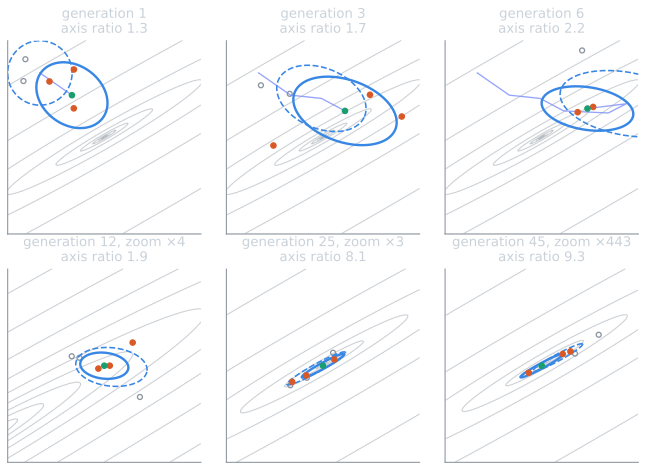
Over more generations. Continuing the same run, the axis ratio was 2.13 after 5 generations, 4.30 after 20, 8.54 after 30 and 11.15 after 60, by which time the long axis pointed at 29.4°, within a degree of the valley, and $f(\mathbf{m})$ was $2.9 \times 10^{-10}$. The mean first reached $f \le 10^{-8}$ in generation 50, after 300 evaluations. With the rank-one update switched off it took 83 generations, with the rank-μ update switched off 59, and with $\sigma$ held fixed at 1 also 83; in the last case the covariance matrix shrinks to do the step size's job, more slowly.
Invariance and the inverse Hessian
CMA-ES behaves identically on whole classes of functions, which is what lets results on a few test functions generalize (Hansen, 2016, §5). Beyond translation, it is invariant to:
- Strictly increasing transformations of $f$. Only the ranking is used, so minimizing $f$, $f^3$ or $e^f$ gives the same sequence of points.
- Rotations and reflections of the search space, provided the initial mean is transformed accordingly.
- Any invertible linear transformation $\mathbf{A}$ of the search space, provided the initial covariance matrix is $\mathbf{A}^{-1}(\mathbf{A}^{-1})^\top$ and the initial mean is transformed with it.
In practice the linear invariance holds only after the algorithm has learned the transformation, since it starts from $\mathbf{C} = \mathbf{I}$. That learning is the point of the method. On a convex quadratic $f(\mathbf{x}) = \frac{1}{2}\mathbf{x}^\top \mathbf{H}\mathbf{x}$, sampling with $\mathbf{C} = \mathbf{H}^{-1}$ is equivalent to optimizing the sphere with $\mathbf{C} = \mathbf{I}$, since the substitution $\mathbf{x} = \mathbf{H}^{-1/2}\mathbf{u}$ turns the ellipsoid into $\frac{1}{2}\mathbf{u}^\top\mathbf{u}$. Hansen (2016, §0.4) therefore takes the inverse Hessian, up to a scalar factor, as the target of covariance adaptation, noting that the intuition and the empirical evidence are strong but a rigorous proof that it is optimal is missing. Learning it is analogous to what a quasi-Newton method such as BFGS does from gradients, except that CMA-ES uses only rankings of function values.
The script below checks this on the ellipsoid. With Hessian $\mathbf{H} = \mathrm{diag}(2 \cdot 10^{6(i-1)/9})$, the matrix $\mathbf{C}^{1/2}\mathbf{H}\mathbf{C}^{1/2}$ would have condition number 1 if $\mathbf{C}$ were exactly proportional to $\mathbf{H}^{-1}$, and $10^6$ if $\mathbf{C}$ were still the identity. At the end of the 30 runs its median condition number is 3.14 (maximum 4.10): the algorithm has removed all but a factor of about three of the original millionfold ill-conditioning. The rotated ellipsoid costs the same number of evaluations as the axis-parallel one, because nothing in the algorithm refers to the coordinate axes.
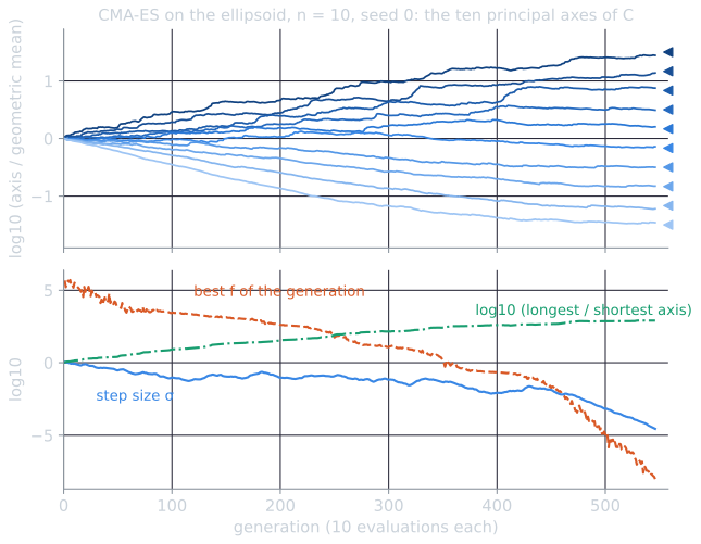
The figure shows where the evaluations go. In this run the ratio of the longest to the shortest axis of $\mathbf{C}$ was 2.6 after 50 generations, 34 after 200, 397 after 400, and 802 at generation 546, when the target was reached after 5,460 evaluations. Most of the run is spent learning the shape; only the last hundred or so generations, after the shape is nearly right, converge at the speed the sphere allows.
Measured behavior
The script tools/experiments/evolution/cmaes.py in the site repository implements the algorithm above in about 100 lines of numpy, with the parameters of the table and positive weights only. Each run uses its own seeded generator, starts from $\mathbf{m}_0$ drawn uniformly from $[-2, 2]^{10}$ with $\sigma_0 = 0.3 \times 4 = 1.2$, and counts evaluations until some sampled point has $f \le 10^{-8}$, within a budget of $10^5$. Over seeds 0 to 29:
| Function ($n = 10$) | Runs reaching $10^{-8}$ | Evaluations, median [IQR] | Range |
|---|---|---|---|
| Sphere $\sum x_i^2$ | 30/30 | 1,344 [1,314, 1,379] | 1,180 to 1,451 |
| Ellipsoid, condition $10^6$ | 30/30 | 5,628 [5,469, 5,694] | 5,273 to 5,982 |
| Same ellipsoid, rotated | 30/30 | 5,519 [5,416, 5,746] | 5,080 to 6,015 |
| Rosenbrock | 29/30 | 5,991 [5,625, 6,294] | 4,823 to 7,228 |
The ellipsoid costs about four times as much as the sphere. The difference is the price of learning $\mathbf{C}$, which starts as the identity; with $\mathbf{C}$ proportional to $\mathbf{H}^{-1}$ from the start, the ellipsoid would behave exactly like the sphere. On Rosenbrock's function, $\sum_{i=1}^{n-1} 100(x_i^2 - x_{i+1})^2 + (1 - x_i)^2$, one run (seed 16) converged to the function's other local minimum, near $(-1, 1, \dots, 1)$ with $f = 3.99$. Step-size control prevents premature convergence, but not convergence to a local optimum (Hansen, 2016, §5).
What each update contributes
The script cmaes_components.py reruns the same 30 starts with parts of the algorithm switched off: the rank-one update ($c_1 = 0$), the rank-μ update ($c_\mu = 0$), the cumulation of $\mathbf{p}_c$ ($c_c = 1$, so the rank-one update sees only the current step and loses its sign), or both covariance updates, which leaves a $(\mu/\mu_W, \lambda)$-ES with cumulative step-size adaptation and $\mathbf{C} = \mathbf{I}$. Evaluations to $f \le 10^{-8}$ in ten dimensions, median [IQR]; all 30 runs reached the target in every cell except the last row:
| Variant | Sphere, $\lambda = 10$ | Ellipsoid, $\lambda = 10$ | Sphere, $\lambda = 50$ | Ellipsoid, $\lambda = 50$ |
|---|---|---|---|---|
| Full | 1,344 [1,314, 1,379] | 5,628 [5,469, 5,694] | 3,958 [3,880, 4,095] | 8,460 [8,260, 8,719] |
| Rank-μ only | 1,375 [1,353, 1,436] | 10,254 [9,879, 10,587] | 4,094 [3,908, 4,164] | 9,346 [9,087, 9,648] |
| Rank-one only | 1,351 [1,326, 1,402] | 7,999 [7,809, 8,118] | 5,095 [4,972, 5,200] | 28,674 [28,295, 29,148] |
| No cumulation of $\mathbf{p}_c$ | 7,769 [7,141, 8,230] | 8,837 [8,594, 9,001] | ||
| No covariance adaptation | 1,422 [1,388, 1,512] | 0/30 within $10^5$ | 5,309 [5,152, 5,425] | 0/30 within $2 \times 10^5$ |
The ellipsoid columns show the division of labor that Hansen (2016, §3.4) describes. With the default $\lambda = 10$, the rank-one update matters more: removing it nearly doubles the cost (10,254 against 5,628), while removing the rank-μ update costs 42%. With $\lambda = 50$ the roles reverse: the rank-μ update alone is within 11% of the full algorithm, and the rank-one update alone needs more than three times as many evaluations, because a large population carries much more information per generation than a single path vector can hold. Cumulation is worth 38% at $\lambda = 10$ and about 4% at $\lambda = 50$, again because it matters most when each generation says little. Without covariance adaptation no run solved the ellipsoid, the case of the 1/5 rule and of single step sizes in self-adaptation. On the sphere, where the identity is already the right shape, every variant at $\lambda = 10$ is within 6% of the full algorithm. At $\lambda = 50$ the two variants without the rank-μ update were about 30% slower. Our reading, not tested further here, is that the rank-μ update with a large population also rescales $\mathbf{C}$ as a whole and so assists the step-size control, which with $\lambda = 50$ in ten dimensions keeps $\sigma$ larger than optimal (compare the experiment on cumulative step-size adaptation in self-adaptation).
As a check against the reference behavior, the script's --reference option reruns the same starts with pycma 4.5.0, Hansen's Python package. Its purecma module, which also uses positive weights only but a slightly different damping, a $c_\mu$ without the $1/4$ term of the table (0.0202 instead of 0.0236 for $n = 10$), and a squared-norm form of the step-size rule, needs medians of 1,475, 5,910 and 6,310 evaluations on the sphere, ellipsoid and Rosenbrock, with 29 of 30 Rosenbrock runs succeeding. The full cma.CMAEvolutionStrategy, with negative weights, needs 1,405, 4,005 and 5,275, with 28 of 30. Both count whole generations, which adds about half a generation (5 evaluations) to their medians compared with the per-evaluation count used here. On the sphere and Rosenbrock, the medians here are within 10% of purecma's and within 14% of the full package's. On the ellipsoid, the full package, whose defaults include active covariance adaptation, needs about 30% fewer evaluations than either positive-weight version.
Restarts with increasing population size
The default population is small, which makes CMA-ES fast and local. On multimodal functions with many regular local minima, such as Rastrigin's function $10n + \sum_{i=1}^n (x_i^2 - 10\cos 2\pi x_i)$, a larger population samples more of the search space in each generation, and Hansen and Kern (2004) found that increasing $\lambda$ improved performance on such functions. Auger and Hansen (2005) turned this into a restart strategy, IPOP-CMA-ES: whenever a run meets one of a set of stopping criteria, a new, independent run starts from a fresh uniform point with the population size doubled. The criteria detect stagnation and numerical trouble: the best values of the last $10 + \lceil 30n/\lambda \rceil$ generations no longer differ, the step size has fallen below a tolerance in every coordinate, adding a tenth of a standard deviation along a principal axis or a fifth along a coordinate no longer changes the mean, or the condition number of $\mathbf{C}$ exceeds $10^{14}$. On the 25 functions of the CEC 2005 benchmark, they compared IPOP with restarts at a constant small population: the two performed similarly on unimodal functions, and on multimodal functions IPOP was significantly better in 29 of 60 cases and significantly worse in 4.
The script reproduces the idea on Rastrigin's function in 10 dimensions, starting from $[-5.12, 5.12]^{10}$ with $\sigma_0 = 5.12$, the CEC 2005 budget of $10^4 n = 10^5$ evaluations, and a subset of Auger and Hansen's stopping criteria. A single run with the default $\lambda = 10$ never reaches $f \le 10^{-8}$: none of the 30 runs does, and their best values have a median of 11.9, the mark of a local minimum. With IPOP restarts, 28 of 30 runs reach the global minimum, after a median of 83,464 evaluations [IQR 51,101 to 87,386]. The successful runs found it with $\lambda = 80$ in one case, $\lambda = 160$ in 12, and $\lambda = 320$ in 15.
A later variant, BIPOP-CMA-ES (Hansen, 2009), splits the budget between two interlaced restart regimes, one with increasing population sizes as in IPOP and one with varying small populations.
Standing in black-box benchmarking
The BBOB workshop at GECCO 2009 benchmarked 31 algorithms on 24 noiseless functions in up to 40 dimensions, with runtime measured in function evaluations. Hansen, Auger, Ros, Finck, and Pošík (2010), the benchmark's organizers, among them the designer of CMA-ES, report that the best choice depends strongly on the budget. For budgets below $500n$ evaluations, the best performers were NEWUOA, MCS, and GLOBAL; for larger budgets, BIPOP-CMA-ES and IPOP-SEP-CMA-ES became superior. In two dimensions, a Nelder-Mead variant was clearly best overall. Wierstra et al. (2014) later used the same benchmark for xNES and took BIPOP-CMA-ES, which they call the winner of the 2009 edition, as the reference point; in the direct comparison they report, xNES with adaptation sampling was significantly better on 6 functions and significantly worse on 18.
The fair summary is that restart variants of CMA-ES are among the strongest general-purpose methods for continuous black-box optimization when the budget is moderate to large, in the low to moderate dimensions those benchmarks cover. They are not the best choice everywhere: in the same benchmark, small budgets favored NEWUOA, MCS and GLOBAL, and two-dimensional problems a Nelder-Mead variant, and the no free lunch theorems rule out a universal winner over all problems.
Against the binary GA of the course assignment
The course's second assignment ran a binary genetic algorithm on De Jong's test functions, including Rosenbrock's function in two dimensions on $[-2.048, 2.048]^2$, with a population of 20 for 50 generations: 1,000 evaluations. The article on that assignment reran the GA over 30 seeds. Its best value had a median of 0.053 [IQR 0.013 to 0.207] with 8 bits per variable and 0.125 [0.031 to 0.351] with 16 bits, and the 8-bit grid cannot represent any point better than 0.0016.
The script gives CMA-ES the same function, box and budget: $n = 2$, so $\lambda = 6$, $\mathbf{m}_0$ uniform in the box, $\sigma_0 = 0.3 \times 4.096$, and 166 generations, 996 evaluations. Over 30 seeds the best value has a median of $7.0 \times 10^{-24}$ [IQR $3.1 \times 10^{-27}$ to $9.2 \times 10^{-21}$]; 29 runs reach $10^{-8}$, after a median of 525 evaluations, and the last ends at $5.8 \times 10^{-8}$. Every run's best point lies inside the box, although the script imposes no bounds.
The gap is large, but the comparison is not a contest between equals, and it should be read with its differences stated:
- Representation. The GA searches a grid of bit strings decoded into the box, with Hamming cliffs between some neighboring values (see binary encoding and Gray codes); CMA-ES samples real vectors at floating-point precision.
- Operators. The GA used fitness-proportionate selection on $1/(f+1)$, which loses pressure as values approach zero, two-point crossover, bit-flip mutation at a fixed rate, and no elitism, all fixed by the assignment. CMA-ES adapts its step size and shape every generation.
- Dimension. Two variables is a small problem. The 10-dimensional results above are a different experiment, and in 2-D the BBOB comparison found a Nelder-Mead variant best overall.
What the comparison shows is the value of matching the representation and the variation operator to a continuous problem and adapting the mutation distribution as the search proceeds, not that one family of evolutionary algorithms is better than the other. A real-coded GA with operators such as those in crossover and mutation operators could narrow the gap; this article does not test that.
Limitations
- Cost per evaluation. Storing $\mathbf{C}$ takes $O(n^2)$ memory, and the eigendecomposition $O(n^3)$ time. Postponing the decomposition for about $1/(10n(c_1 + c_\mu))$ generations reduces the internal effort to $O(n^2)$ per sampled point (Hansen, 2016, App. B.2). Separable variants, which adapt only the diagonal, trade the ability to learn rotations for linear cost; the separable natural evolution strategy is one.
- Noise. Path-length control can fail to find good step sizes on very noisy functions (Hansen, 2016, §4).
- Local optima. A single run is a local search with a large, adaptive neighborhood. Restarts, larger populations, or problem knowledge are needed on rugged fitness landscapes, as the Rosenbrock failure and the Rastrigin runs above show.
CMA-ES also has a reading as gradient ascent: without its evolution paths, its updates of the mean and covariance approximately follow the natural gradient of expected fitness with respect to the parameters of the search distribution (Akimoto, Nagata, Ono, and Kobayashi, 2010). That connection, and the simpler evolution strategies used to train neural networks, are the subject of natural evolution strategies.
References
- Akimoto, Y., Nagata, Y., Ono, I., and Kobayashi, S. (2010). Bidirectional relation between CMA evolution strategies and natural evolution strategies. In Parallel Problem Solving from Nature, PPSN XI, Lecture Notes in Computer Science 6238, 154–163. Springer.
- Auger, A., and Hansen, N. (2005). A restart CMA evolution strategy with increasing population size. In Proceedings of the 2005 IEEE Congress on Evolutionary Computation, vol. 2, 1769–1776.
- Hansen, N. (2009). Benchmarking a BI-population CMA-ES on the BBOB-2009 function testbed. In Proceedings of the 11th Annual Conference Companion on Genetic and Evolutionary Computation (GECCO 2009), 2389–2396.
- Hansen, N. (2016). The CMA evolution strategy: A tutorial. arXiv:1604.00772 (version 2, 2023).
- Hansen, N., Auger, A., Ros, R., Finck, S., and Pošík, P. (2010). Comparing results of 31 algorithms from the black-box optimization benchmarking BBOB-2009. In Proceedings of the 12th Annual Conference Companion on Genetic and Evolutionary Computation (GECCO 2010), 1689–1696.
- Hansen, N., and Kern, S. (2004). Evaluating the CMA evolution strategy on multimodal test functions. In Parallel Problem Solving from Nature, PPSN VIII, Lecture Notes in Computer Science 3242, 282–291. Springer.
- Hansen, N., Müller, S. D., and Koumoutsakos, P. (2003). Reducing the time complexity of the derandomized evolution strategy with covariance matrix adaptation (CMA-ES). Evolutionary Computation, 11(1), 1–18.
- Hansen, N., and Ostermeier, A. (1996). Adapting arbitrary normal mutation distributions in evolution strategies: the covariance matrix adaptation. In Proceedings of the 1996 IEEE International Conference on Evolutionary Computation, 312–317.
- Hansen, N., and Ostermeier, A. (2001). Completely derandomized self-adaptation in evolution strategies. Evolutionary Computation, 9(2), 159–195.
- Jastrebski, G. A., and Arnold, D. V. (2006). Improving evolution strategies through active covariance matrix adaptation. In Proceedings of the 2006 IEEE International Conference on Evolutionary Computation, 2814–2821.
- Wierstra, D., Schaul, T., Glasmachers, T., Sun, Y., Peters, J., and Schmidhuber, J. (2014). Natural evolution strategies. Journal of Machine Learning Research, 15, 949–980.