A robot navigating a maze is scored by how close it ends to the goal. Most of the maze rewards that score honestly, but one corridor heads straight at the goal and stops at a wall, and the real route starts by leading away. A genetic algorithm that selects on distance to the goal fills its population with robots pressed against that wall, because every step down the true route makes the score worse before it makes it better. Running longer does not help. The fitness function itself points the wrong way.
Now consider a different request: not the single best controller for a robot arm, but a reachable configuration for every point the arm can touch, each one as comfortable as possible for that point. A search that returns one excellent configuration has answered the wrong question, however good the configuration is.
Both cases ask search to value difference, not only quality. Novelty search rewards behavior that has not been seen before and ignores the objective entirely. Quality-diversity (QD) algorithms, of which MAP-Elites is the simplest and most widely used, keep the best solution found for each kind of behavior. This article covers both, the measures used to compare them, an extension for many behavior dimensions, the best-known application, and an experiment that shows on a small benchmark what the archive buys and what it costs.
Deception and the search for novelty
Lehman and Stanley introduced novelty search in 2008 and gave its fullest account in a journal paper (Lehman and Stanley, 2008, 2011). Their test was the maze above. A wheeled robot, controlled by a neural network evolved with NEAT, has a fixed time to travel from start to goal. The objective-based version scores a robot by $f = b_f - d_g$, where $d_g$ is its distance to the goal at the end of the run and $b_f$ is a constant that keeps scores positive. On a "hard" map, built so that the fitness gradient leads into a dead end, the results over 40 runs were:
| Method | Hard map solved | Medium map solved | Medium map, mean evaluations to solve |
|---|---|---|---|
| NEAT, fitness $b_f - d_g$ | 3 of 40 | 40 of 40 | 56,334 |
| NEAT, random selection | 4 of 40 | 21 of 40 | not reported |
| NEAT, novelty search | 39 of 40 | 40 of 40 | 18,274 |
A robot counted as a solution if it ended within five units of the goal, and runs were capped at 250,000 evaluations. On the hard map, selection on fitness did no better than selecting at random, which is what deception means in practice: the information the objective gives is misleading, not merely weak. On the medium map, where both methods always succeeded, novelty search needed about a third as many evaluations on average (Lehman and Stanley, 2011, §6).
How novelty is measured
Novelty search needs two things the objective does not supply.
The first is a behavior characterization: a description of what a candidate does, chosen by the experimenter. In the maze it was the robot's final position, two numbers, ignoring the path taken. Many different networks collapse to the same behavior, which is what keeps the space of behaviors small enough to explore.
The second is a measure of how unusual a behavior is. Lehman and Stanley used sparseness, the average distance from a behavior $x$ to its $k$ nearest neighbors:
$$\rho(x) = \frac{1}{k} \sum_{i=1}^{k} \operatorname{dist}(x, \mu_i),$$
where $\mu_i$ is the $i$-th nearest neighbor of $x$ among the current population and an archive of past behaviors, and $\operatorname{dist}$ is a domain-specific behavioral distance (in the maze, the squared Euclidean distance between end points). A candidate whose sparseness exceeds a threshold $\rho_{\min}$ is added to the archive permanently. The archive is the search's memory: without it, a population rewarded only for differing from itself can drift back and forth over the same ground. The maze runs used $k = 15$, a population of 250, and an initial value of 6.0 for the archive threshold (Lehman and Stanley, 2011, Appendix A). Selection then proceeds as in any evolutionary algorithm, with novelty in place of fitness, and the objective is checked only to decide when to stop.
A small example shows the computation. Take $k = 3$, plain Euclidean distance, and an archive of five end points in a maze: $(1,1)$, $(2,1)$, $(1,3)$, $(3,2)$ and $(6,1)$. (In a real run the current population is searched too; leaving it out keeps the arithmetic short.) Two new robots end at $P = (2,2)$ and $Q = (8,3)$:
| Archived end point | Distance to $P = (2,2)$ | Distance to $Q = (8,3)$ |
|---|---|---|
| $(1,1)$ | 1.414 | 7.280 |
| $(2,1)$ | 1.000 | 6.325 |
| $(1,3)$ | 1.414 | 7.000 |
| $(3,2)$ | 1.000 | 5.099 |
| $(6,1)$ | 4.123 | 2.828 |
| Mean of the 3 nearest (bold) | $\rho(P) = 1.138$ | $\rho(Q) = 4.751$ |
($P$ has two neighbors tied at 1.414; either one gives the same mean.) $P$ lands in the crowded corner where the archive already has four points, so its sparseness is small. $Q$ lands where only one point is nearby, so even its third-nearest neighbor is far away. With a threshold $\rho_{\min} = 3$, $Q$ would join the archive and $P$ would not, and in selection $Q$ would be preferred to $P$ whether or not either is closer to the goal. Once $Q$ is archived, a later robot ending near $(8,3)$ scores lower than $Q$ did, which is how the archive pushes the search onward. The numbers are computed by tools/experiments/evolution/novelty_maze.py (rounded to three decimals).
Novelty search is not a random walk. The archive pushes the search away from where it has already been, and the 21-of-40 success rate of random selection on the medium map, against 40 of 40 for novelty, shows the difference.
The deceptive maze in miniature
The effect can be reproduced in a few hundred lines of code. Our version, tools/experiments/evolution/novelty_maze.py, simplifies the robot: instead of a neural network with sensors, a genome is an open-loop path of 20 headings, each moving a point robot 2 units, with the robot sliding along any wall it runs into. The behavior is the end point. The maze is a 10 by 10 box with two internal walls. The robot starts at the bottom left and the goal is at the top right. Heading toward the goal leads through the gap on the right of the lower wall into a corridor that ends under the upper wall, 2.65 units from the goal: the dead end. The real route turns back west along the corridor, which takes the robot almost 9 units from the goal, then up through the gap on the left and east again.
The three methods differ only in the score used for selection: closeness to the goal, sparseness ($k = 15$, Euclidean distance, an archive with an adaptive threshold), or a random number. Each is a generational algorithm with population 100, binary tournaments, Gaussian mutation of the headings and one elite, and stops on reaching the goal or after 30,000 evaluations. Over 30 seeded runs each:
| Selection by | Runs that reached the goal | Evaluations to reach it, median [Q1, Q3] of successful runs | Where unsolved runs ended |
|---|---|---|---|
| Fitness (distance to goal) | 9 of 30 | 6,900 [5,100, 12,000] | 19 of 21 within 0.2 of the dead end |
| Novelty | 27 of 30 | 9,400 [4,750, 18,600] | elsewhere (none at the dead end) |
| Random | 0 of 30 | closest robot a median 3.15 from the goal |
Fitness-based search either found the route early, before its population had collapsed onto the dead end, or never found it. In 19 of the 21 unsolved fitness runs, the robot closest to the goal at the end was 2.65 units away, pressed into the corner of the dead end. Novelty search solved nine runs in ten, and none of its three failures ended at the dead end: once the archive held robots there, ending there earned nothing. Random selection, with the same mutation and the same budget, never reached the goal, and its closest robots ended a median 3.15 units away, which is the other half of Lehman and Stanley's point: novelty search is not undirected.
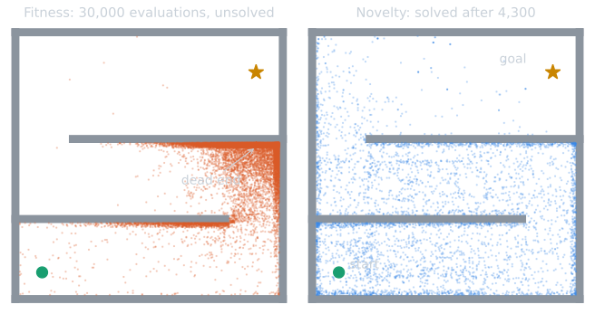
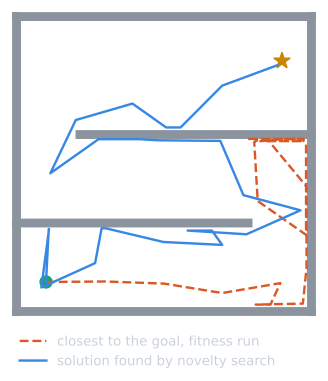
The numbers are ours, on a simplified task, and the success rates depend on the budget and the maze. The pattern is the one Lehman and Stanley reported: the objective pulls the population into the place that looks closest, and a search that ignores the objective finds the goal more reliably.
Where novelty search fails
The same paper reports its limits.
- Unbounded behavior spaces. With two outer walls removed, robots could wander into open space, and novelty search solved the maze only 5 times in 100 runs, against 2 for fitness-based search. Every new place outside the maze counts as novel, so learning to navigate within it earns nothing special. The behavior characterization has to make the interesting behaviors a small part of the space.
- Cost. Each novelty score requires a nearest-neighbor search over population and archive, which grows as the archive grows. In the hard maze, an archive capped at 250 entries (a queue that drops the oldest) still solved all 40 runs, so in this domain the memory could be bounded without loss.
In a biped walking task, novelty search evolved gaits that traveled 4.04 m on average in 15 simulated seconds, against 2.88 m for fitness-based search, over 50 runs (Lehman and Stanley, 2011, §8). Novelty search is not limited to small mazes, but its success depends on a characterization in which the goal is a reachable kind of novelty.
From novelty to quality diversity
Pure novelty search discards quality. For a robot that must walk, it returns many different gaits with no guarantee that any of them is a good example of its kind. Lehman and Stanley's follow-up, novelty search with local competition, kept two objectives: novelty, and performance compared only against a candidate's 15 nearest neighbors in behavior space, so that a slow but unusual gait competes with similar gaits and not with the fastest one overall (as described by Mouret and Clune, 2015, §4).
Pugh, Soros, Szerlip and Stanley (2015) named the resulting family. In the words of Pugh, Soros and Stanley (2016), the goal of quality diversity is "to find a maximally diverse collection of individuals (with respect to a space of possible behaviors) in which each member is as high performing as possible." This differs from two older goals:
- Diversity for the sake of optimization. Fitness sharing, crowding, island models and speciation keep a population varied so that it does not converge too early, but they are still judged by the best solution found (Eiben and Smith, 2015, §5.5). Multimodal optimization goes further and wants every peak of the fitness function, but still only the peaks.
- Multi-objective optimization. A Pareto front holds the best trade-offs between objectives. A QD archive holds the best solution for each behavior, including behaviors that are dominated everywhere: the best gait that uses only three legs is worth keeping even if it is slower than every four-legged gait.
MAP-Elites
Mouret and Clune (2015) proposed MAP-Elites, short for Multi-dimensional Archive of Phenotypic Elites, as an illumination algorithm: one that returns the highest-performing solution it can find at each point of a space of features chosen by the user, and so illuminates how performance varies across that space.
The user supplies a performance function $f(x)$ for a candidate $x$, a feature descriptor (behavior characterization) $b(x)$ with $N$ dimensions, and a discretization of each dimension, so that the feature space becomes a grid of cells. The archive holds at most one solution per cell, its elite, along with the elite's performance. The simple default version runs as follows (Mouret and Clune, 2015, Fig. 2):
- Start with an empty grid.
- For each of $I$ iterations:
- For the first $G$ iterations, generate a random candidate $x'$.
- Afterwards, pick an occupied cell uniformly at random and create $x'$ by mutating (and possibly crossing over) its elite.
- Evaluate $x'$, recording $p' = f(x')$ and $b' = b(x')$, and find the cell containing $b'$.
- If that cell is empty, or its elite's performance is less than $p'$, store $x'$ and $p'$ there, discarding the old elite.
- Return the grid of elites and their performances.
There is no population apart from the archive, no novelty score, and no comparison between cells. Selection is uniform over occupied cells, so a modest solution in a sparsely visited region is as likely to become a parent as the best solution in the archive. Competition happens only within a cell. The algorithm stops when the budget runs out, never because it has converged, and the number of cells and their elites are its whole state, which makes runs easy to inspect and to compare.
The algorithm has the parameters of its variation operator, the initial sample size $G$, and the grid resolution. The resolution is the consequential choice. Cells that are too large merge behaviors the user wanted separated; cells that are too small spread the budget over more elites than it can improve.
Measuring an archive
A single best value says little about a QD algorithm. The common measures are:
- Coverage: the fraction of cells that hold an elite. It ignores quality. Some cells may be unreachable, so coverage is sometimes reported against the cells that any method has filled.
- QD-score: the sum, over occupied cells, of the elite's performance, introduced by Pugh, Soros, Szerlip and Stanley (2015) and used as the main measure by Pugh, Soros and Stanley (2016). It rewards both filling cells and improving them. It assumes non-negative performance; with negative values, an extra cell could lower the score, so performance is shifted by a constant first.
- Best single solution: the measure an optimizer would be judged on.
Mouret and Clune (2015, §5) also defined global reliability, the average over cells of each elite's performance divided by the best performance any run found in that cell, with empty cells counted as zero and cells that no run filled left out, which is closely related to a normalized QD-score.
To compare a QD algorithm with an ordinary optimizer, Mouret and Clune recorded every candidate the optimizer evaluated and kept the best per cell, as though the optimizer had kept an archive without using it. The experiment below does the same.
An experiment: the planar robotic arm
The arm benchmark comes from the QD literature (Cully, Clune, Tarapore, and Mouret, 2015; Vassiliades and Mouret, 2018). A planar arm has $n = 12$ revolute joints with no limits and links of length $1/n$, so its end effector can reach every point of the unit disk. A candidate is a vector of joint angles $y \in [-\pi, \pi]^{12}$, and its behavior is the end-effector position given by forward kinematics:
$$b(y) = \left( \sum_{i=1}^{n} \tfrac{1}{n} \cos(y_1 + \dots + y_i),\; \sum_{i=1}^{n} \tfrac{1}{n} \sin(y_1 + \dots + y_i) \right).$$
The performance is the negative variance of the joint angles, which favors smooth configurations in which every joint bends by nearly the same angle:
$$f(y) = -\frac{1}{n} \sum_{i=1}^{n} (y_i - \bar{y})^2, \qquad \bar{y} = \frac{1}{n} \sum_{i=1}^{n} y_i.$$
Every reachable point has some best configuration, so a full archive is a lookup table for inverse kinematics, one solution per region of the workspace. For the QD-score we use $q = 1 + f/\pi^2$, which lies in $[0, 1]$ because angles in $[-\pi, \pi]$ have variance at most $\pi^2$, and which orders solutions exactly as $f$ does.
A worked configuration makes the two formulas concrete. Let the joints alternate between bending $+0.3$ and $-0.3$ radians. The running sums $y_1 + \dots + y_i$ are then $0.3, 0, 0.3, 0, \dots$, six of each, so
$$b = \left(\tfrac{6}{12}\cos 0.3 + \tfrac{6}{12}\cos 0,\; \tfrac{6}{12}\sin 0.3 + \tfrac{6}{12}\sin 0\right) = (0.9777,\ 0.1478).$$
The angles have mean 0 and variance $0.3^2 = 0.09$, so $f = -0.09$ and $q = 1 - 0.09/\pi^2 = 0.9909$. On the 50 by 50 grid the cell index along each axis is $\lfloor (b + 1)/2 \times 50 \rfloor$, which puts this arm in column 49, row 28: the last column, at the right edge of the disk, just above the horizontal axis. Any other configuration that ends in the same cell competes with this one for it, and the one with the smaller joint-angle variance keeps it.
What $q = 1$ means geometrically is worth seeing. Zero variance means every joint bends by the same angle $\alpha$, so the arm lies along a circular arc: straight when $\alpha = 0$, curled into a closed regular 12-gon when $\alpha = 30^\circ$, since $12 \times 30^\circ = 360^\circ$ brings the end effector back to the base. As $\alpha$ grows from 0 to $30^\circ$ the end point traces a spiral from $(1, 0)$ into the origin; at $\alpha = 15^\circ$ it is at $(-0.0833, 0.6330)$. Only the cells on that curve can hold a perfect arm. Every other cell must be reached by joints that bend unequally, so its best possible $q$ is below 1. That is why the elites in the figure below have different qualities even after a long run: the archive records the best compromise available at each point, not a uniform standard.
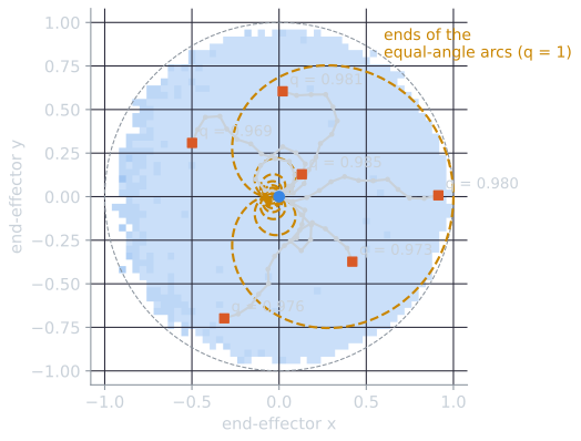
The setup, our own within the published benchmark:
- Genotype and archive. Genotypes lie in $[0, 1]^{12}$ and map to angles by $y = 2\pi(x - 0.5)$. The archive is a 50 by 50 grid over $[-1, 1]^2$. Of its 2,500 cells, 2,052 intersect the unit disk, which bounds the coverage any method can reach at 0.8208.
- MAP-Elites. Exactly as above, in batches of 100: 1,000 random genotypes, then repeated batches of 100 parents drawn uniformly from the filled cells. Mutation is Gaussian, $x' = \mathrm{clip}(x + \mathcal{N}(0, 0.1^2 I), 0, 1)$, the isotropic operator Vassiliades and Mouret (2018) used as a baseline.
- GA. A generational genetic algorithm that maximizes $q$: population 100, binary tournament selection, the same mutation, no crossover, and elitism of one. Every genotype it evaluates is offered to a grid archive used only for measurement.
- Random sampling. Uniform random genotypes, also archived.
- Budget. 100,000 evaluations per run and 30 seeds per method.
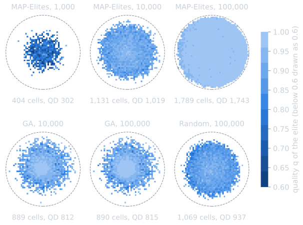
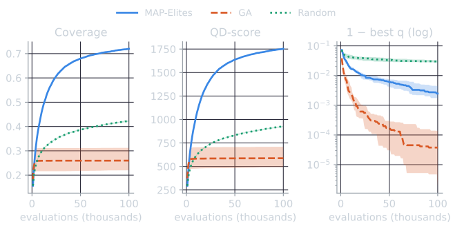
Results after 100,000 evaluations, median and interquartile range over the 30 seeds:
| Method | Coverage | Filled cells (median) | QD-score | Mean $q$ of elites | Best $q$ |
|---|---|---|---|---|---|
| MAP-Elites | 0.7200 [0.7166, 0.7212] | 1,800 | 1,753 [1,745, 1,756] | 0.9739 | 0.9975 [0.9955, 0.9983] |
| GA | 0.2596 [0.2198, 0.3120] | 649 | 588 [492, 710] | 0.9049 | 1.0000 [0.9999, 1.0000] |
| Random sampling | 0.4226 [0.4197, 0.4256] | 1,056.5 | 927 [920, 932] | 0.8765 | 0.9704 [0.9674, 0.9742] |
What the runs show (our observations on this benchmark):
- MAP-Elites fills most of the reachable workspace. Its 1,800 cells are 88% of the 2,052 that intersect the disk, against 32% for the GA. MAP-Elites had the higher coverage and QD-score in all 30 paired seeds at 50,000 and 100,000 evaluations, and in 29 of 30 at 10,000.
- The GA stops exploring. Its coverage was 0.2592 after 10,000 evaluations and 0.2596 after 100,000. Almost all the cells it touched were visited before the population converged, and by 10,000 evaluations it had covered less of the grid than random sampling, which kept spreading.
- The GA finds the best single arm. A variance of zero means every joint has the same angle, which the GA approaches (best $q$ 1.0000 at four decimals). MAP-Elites' best was 0.9975, a joint-angle variance of about 0.025 rad². The GA's best was at least as good as MAP-Elites' in 29 of 30 seeds at 100,000 evaluations, and in every seed at 10,000 and 50,000.
- The archive's elites are good, not just present. The mean $q$ of MAP-Elites' elites rose from 0.9001 at 10,000 evaluations to 0.9739 at 100,000, while the cells filled grew from 0.4596 to 0.7200 of the grid, so the budget went both to new cells and to improving old ones.
The trade is the one the QD framing predicts. An optimizer spends its budget on one region and does best there; MAP-Elites spreads the budget and returns a usable configuration for most of the workspace. The arm is a mild problem, smooth and cheap, and the ranking of methods depends on the measure chosen: by best single solution, the GA wins. The script is tools/experiments/evolution/map_elites.py in the site repository.
The demo below runs the same three methods on the same arm in the browser. Choose a method and press the buttons to spend the budget a thousand evaluations at a time, or run straight to 100,000; tap a filled cell to draw the elite arm stored there. It draws its random numbers from a different generator than the script, so a single run will not reproduce the table, but over 30 seeds its medians at 100,000 evaluations (coverage 0.7196 for MAP-Elites, 0.2406 for the GA, 0.4210 for random sampling) fall inside the interquartile ranges above. Two things are worth trying: run the GA and watch the filled region stop growing once the population has converged, and in a finished MAP-Elites archive compare the elites near the rim, which must be almost straight, with those near the base, which must fold back on themselves.
Scaling the descriptor: CVT-MAP-Elites
A grid with $d$ divisions per dimension has $d^N$ cells, so the archive grows exponentially with the number of descriptor dimensions. Six dimensions at five divisions already give 15,625 cells, and twenty dimensions are out of reach. Vassiliades, Chatzilygeroudis and Mouret (2018) replaced the grid with a centroidal Voronoi tessellation (CVT): $k$ points (centroids) spread evenly over the feature space, each owning the region of points closer to it than to any other centroid. The number of cells is $k$, chosen by the user, whatever the dimension.
They built the tessellation approximately, by sampling many random points in the feature space and running the alternating assign-and-update procedure of K-means on them, which moves the $k$ centroids until they are well spread. The algorithm is otherwise MAP-Elites, with "the cell containing $b'$" replaced by "the region of the nearest centroid." In maze navigation they used descriptors with up to 1,000 dimensions, which no grid could hold, and in hexapod locomotion higher-dimensional descriptors produced faster gaits in their evaluation settings (Vassiliades, Chatzilygeroudis, and Mouret, 2018, §§IV–V).
Robots that adapt like animals
The result that brought QD to wide attention was Cully, Clune, Tarapore and Mouret (2015), in Nature. Their method, Intelligent Trial and Error, has two stages.
- Before deployment, MAP-Elites runs in simulation to build a behavior-performance map: thousands of controllers, each the best found for its kind of behavior, with its simulated performance.
- After damage, the real robot searches the map rather than the controller parameters. Bayesian optimization, using the simulated performances as its prior, chooses which behaviors to try, updates its estimate of the whole map after each physical trial, and stops when a tested behavior reaches 90% of the highest performance the updated map predicts for any behavior, or after 20 physical trials.
The paper reports that the method "allows robots to adapt to damage in less than two minutes," with successful adaptation "for a legged robot injured in five different ways, including damaged, broken, and missing legs, and for a robotic arm with joints broken in 14 different ways" (Cully et al., 2015, abstract). In the authors' manuscript, the six-legged robot's 36 gait parameters were mapped onto a six-dimensional behavior space, the fraction of time each leg touches the ground, at five values per dimension, and a map held about 13,000 gaits. Across the four damage conditions the robot adapted in a median of 66 seconds and 8 physical trials (5th to 95th percentiles 24 to 134 seconds and 3 to 16 trials). The arm in that work was a planar arm with eight joints whose behavior was the end-effector position and whose performance favored low variance of the joint angles, the ancestor of the benchmark above (Cully et al., 2014).
The claim is precise and should be read that way. The robot does not learn a new gait from scratch in two minutes; it selects among gaits found in a long simulated search beforehand, using a few physical trials to discover which of them still work. The map's diversity is what makes this possible: a damaged robot needs gaits that avoid the broken leg, and those are low-performing on an intact robot, so an optimizer would never have kept them. The authors also report that Bayesian optimization run directly in the 36-dimensional parameter space did not find working controllers in the same setting.
Limits and open questions
- The behavior characterization is a design decision. It defines what counts as different, and so what the algorithm explores. The unenclosed maze showed how a poorly constrained characterization defeats novelty search, and a QD archive can only be as useful as its descriptor.
- Evaluations. Robot repertoires typically take a few million evaluations (Vassiliades and Mouret, 2018), affordable in fast simulation and hardly anywhere else. Vassiliades and Mouret's response was a better variation operator: elites in different cells tend to share much of their genotype, so their directional operator samples offspring along the line between two elites, which in their Schwefel-function and arm experiments improved the archive faster than isotropic Gaussian mutation.
- Noise. MAP-Elites keeps whichever candidate scored highest once in each cell. With noisy evaluations, a lucky evaluation can hold a cell indefinitely; the experiment above is deterministic, so this problem does not arise there.
- What diversity is for. Novelty search is often discussed in connection with open-ended evolution, the search for systems that keep producing new things indefinitely, a question taken up under artificial life platforms.
QD ideas have spread into other systems. Evolution through large models used MAP-Elites with a language model as the mutation operator, and the program database of AlphaEvolve draws on MAP-Elites and island models; both are described in AlphaEvolve and LLM-guided evolution. Applications to physical robots are covered in evolutionary robotics.
References
- Cully, A., Clune, J., Tarapore, D., and Mouret, J.-B. (2014). Robots that can adapt like animals. Authors' manuscript, arXiv:1407.3501 (version 4, 2015).
- Cully, A., Clune, J., Tarapore, D., and Mouret, J.-B. (2015). Robots that can adapt like animals. Nature, 521(7553), 503–507.
- Eiben, A. E., and Smith, J. E. (2015). Introduction to Evolutionary Computing, 2nd ed., section 5.5. Springer.
- Lehman, J., and Stanley, K. O. (2008). Exploiting open-endedness to solve problems through the search for novelty. In Artificial Life XI: Proceedings of the Eleventh International Conference on the Simulation and Synthesis of Living Systems, 329–336. MIT Press.
- Lehman, J., and Stanley, K. O. (2011). Abandoning objectives: evolution through the search for novelty alone. Evolutionary Computation, 19(2), 189–223.
- Mouret, J.-B., and Clune, J. (2015). Illuminating search spaces by mapping elites. arXiv:1504.04909.
- Pugh, J. K., Soros, L. B., Szerlip, P. A., and Stanley, K. O. (2015). Confronting the challenge of quality diversity. In Proceedings of the 2015 Genetic and Evolutionary Computation Conference (GECCO), 967–974.
- Pugh, J. K., Soros, L. B., and Stanley, K. O. (2016). Quality diversity: a new frontier for evolutionary computation. Frontiers in Robotics and AI, 3, 40.
- Vassiliades, V., Chatzilygeroudis, K., and Mouret, J.-B. (2018). Using centroidal Voronoi tessellations to scale up the multidimensional archive of phenotypic elites algorithm. IEEE Transactions on Evolutionary Computation, 22(4), 623–630.
- Vassiliades, V., and Mouret, J.-B. (2018). Discovering the elite hypervolume by leveraging interspecies correlation. In Proceedings of the Genetic and Evolutionary Computation Conference (GECCO), 149–156.