A neural network with two inputs, two hidden units and one output has nine adjustable numbers: two incoming weights and a bias for each hidden unit, and two weights and a bias for the output. Fix that structure, and choosing the network is the same as choosing a point in nine-dimensional real space. A genetic algorithm can search that space as it searches any other: treat the nine numbers as a chromosome, score each chromosome by how well its network performs, and breed the better ones. No gradient is computed, so the score can be anything that can be measured, such as how long a controller keeps a pole balanced or how many points an agent earns in a game.
This is the oldest and simplest form of neuroevolution: the topology is chosen by hand and evolution searches only the connection weights. In the traditional setup that Stanley and Miikkulainen (2002) describe, the topology is a single hidden layer with every hidden unit connected to every input and every output, and evolution explores the weights through crossover of weight vectors and mutation of single networks. This article runs that setup on the smallest interesting problem, XOR, and uses it to show the problem that dominated the early literature: two networks can compute the same function with their hidden units in a different order, and crossing them can destroy what both had. It then describes the cooperative methods that worked around the problem and the evidence, from 2017 on, that weight evolution can compete with gradient-based training on some reinforcement learning tasks.
Why evolve weights
Gradient descent with backpropagation needs a differentiable loss and a target for every output. Many problems supply neither. A controller for a robot or a simulated cart receives a single score at the end of an episode, and there is no correct action to compare against at each time step. Neuroevolution needs only that score. Montana and Davis (1989) also pointed out that backpropagation cannot handle discontinuous transfer functions or discontinuous error criteria, which an evolutionary search does not care about, and they argued that gradient search tends to become trapped in local minima of the error surface.
Montana and Davis trained a network with four inputs, two hidden layers of seven and ten units and one output, 126 weights in all, to classify features of passive sonar images. Their genetic algorithm encoded the weights and biases as a list of real numbers, used the sum of squared errors over 236 training examples as the evaluation, and experimented with a range of operators. A version with node-level mutation and crossover outperformed backpropagation on their data, with two genetic algorithm iterations counted as equivalent in computation to one pass of backpropagation. Whitley, Starkweather and Bogart (1990) applied genetic algorithms both to the weights of feed-forward networks and to their connectivity. Yao's (1999) review organizes the field that followed by what is evolved: connection weights, architectures, learning rules and input features. This article covers the first; NEAT and architecture search cover the second.
A seeded experiment: XOR with a fixed 2-2-1 network
XOR is the classic test because a network without hidden units cannot compute it: no single weighted sum of $x_1$ and $x_2$ separates the inputs $(0,1)$ and $(1,0)$ from $(0,0)$ and $(1,1)$. With two hidden units it can. The network here computes
$$h_1 = s(a_1 x_1 + b_1 x_2 + c_1), \quad h_2 = s(a_2 x_1 + b_2 x_2 + c_2), \quad y = s(v_1 h_1 + v_2 h_2 + d),$$
where $s(z) = 1 / (1 + e^{-4.9 z})$ is the steepened sigmoid that Stanley and Miikkulainen (2002) used, so that the task matches the NEAT experiment in the companion article. The genome lists the weights grouped by hidden unit:
$$[a_1, b_1, c_1, \; a_2, b_2, c_2, \; v_1, v_2, d].$$
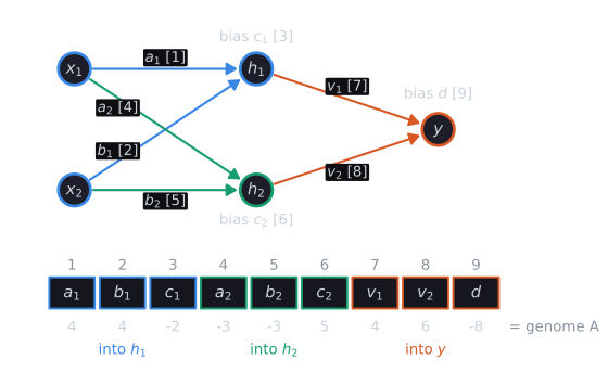
The mapping from genome to network is fixed: position 1 is always the weight from $x_1$ into the first hidden unit, position 7 always the weight from the first hidden unit into the output. That fixity is what lets a standard crossover operator work on the genome without knowing it describes a network, and, as the section on competing conventions shows, it is also the source of the method's main weakness.
Fitness is NEAT's XOR fitness: the absolute errors on the four input patterns are summed, the sum is subtracted from 4, and the result is squared, so a perfect network scores 16. A network counts as solving XOR when every output is on the correct side of 0.5.
One solution worked through
A hand-built genome shows how a 2-2-1 network computes XOR. Take
$$A = [4, 4, -2, \; -3, -3, 5, \; 4, 6, -8].$$
The first hidden unit computes $h_1 = s(4x_1 + 4x_2 - 2)$. Its weighted sum is $-2$ when both inputs are 0 and at least $2$ otherwise, and the steep sigmoid turns those into values near 0 and near 1, so $h_1$ acts as OR. The second computes $h_2 = s(-3x_1 - 3x_2 + 5)$, whose sum is positive unless both inputs are 1, so it acts as NAND. The output $y = s(4h_1 + 6h_2 - 8)$ is near 1 only when both hidden units are near 1, which makes it an AND of the two, and OR AND NAND is XOR. Every value, from tools/experiments/evolution/fixed_topology_worked.py, rounded to four decimals:
| $x_1$ | $x_2$ | $4x_1 + 4x_2 - 2$ | $h_1$ | $-3x_1 - 3x_2 + 5$ | $h_2$ | $4h_1 + 6h_2 - 8$ | $y$ | target |
|---|---|---|---|---|---|---|---|---|
| 0 | 0 | $-2$ | 0.0001 | 5 | 1.0000 | $-1.9998$ | 0.0001 | 0 |
| 0 | 1 | 2 | 0.9999 | 2 | 0.9999 | 1.9994 | 0.9999 | 1 |
| 1 | 0 | 2 | 0.9999 | 2 | 0.9999 | 1.9994 | 0.9999 | 1 |
| 1 | 1 | 6 | 1.0000 | $-1$ | 0.0074 | $-3.9557$ | 0.0000 | 0 |
With the slope of 4.9, $s(2) = 0.99994$, so a weighted sum of 2 is already effectively "on". The NAND unit is the least saturated of the hidden values: at $(1,1)$ its sum is only $-1$, and $h_2 = 0.0074$. The output still has a margin of almost 4 there, because its bias of $-8$ needs both hidden units near 1 to be overcome. The four absolute errors are 0.000056, 0.000056, 0.000056 and essentially 0, summing to 0.000167, and the fitness is $(4 - 0.000167)^2 = 15.9987$.
The same fitness formula explains the trap that the experiment below runs into. A network whose outputs are exactly right on three patterns and exactly wrong on the fourth has a summed error of 1 and a fitness of $(4 - 1)^2 = 9$. OR, with outputs $0, 1, 1, 1$, is such a network, and so is any network that outputs 1 on a single pattern. Since saturated outputs move very little under small weight changes, a network at 9 has few neighbours that score better.
The genetic algorithm, implemented in tools/experiments/evolution/weight_evolution.py in the site repository, is fully specified so that each run is reproducible from its seed:
- a population of 150 genomes, with initial weights drawn uniformly from $[-2, 2]$;
- generational replacement with elitism: the best genome is copied unchanged and 149 children replace the rest;
- each child gets two parents by binary tournament (draw two genomes at random, keep the fitter);
- with probability 0.75 the parents undergo one-point crossover at a cut drawn uniformly from the eight positions between genes, otherwise the child copies the first parent;
- each gene then mutates with probability 0.2 by adding Gaussian noise with standard deviation 0.5;
- a run stops at the first genome that solves XOR, or after 300 generations (45,000 evaluations).
Over 30 seeds:
| Search | Runs solved | Evaluations to solve, median [Q1, Q3] |
|---|---|---|
| GA with crossover | 30 of 30 | 840 [508, 1,320] |
| GA, mutation only | 24 of 30 | 796 [120, 1,238] |
| Random search over $[-2, 2]^9$ | 30 of 30 | 1,050 [235, 1,852] |
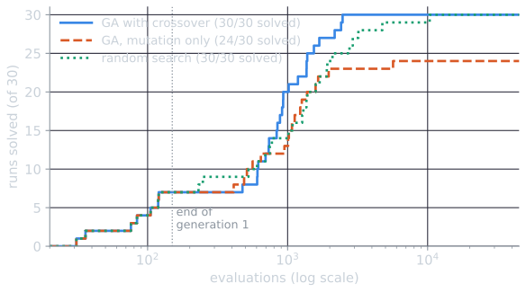
The numbers are a warning about XOR as a benchmark. In 7 of the 30 seeds the initial random population of 150 already contained a solution, and pure random sampling from the same initial distribution found one after a median of 1,050 draws. The curves show the comparison in full: the medians hide that the genetic algorithm with crossover solved every run within 2,470 evaluations, while random search needed 4,750 and 10,341 evaluations in its two slowest runs. With the right topology given and a steep sigmoid, XOR is easy enough that the genetic algorithm's advantage over random search is small. The mutation-only variant failed in 6 runs, and all six ended on the same kind of trap: a best network with fitness 9.0 whose saturated outputs are right on three patterns and fully wrong on the fourth. Three of them compute OR, and the other three output 1 on a single pattern. Such a network computes a different Boolean function exactly, and small mutations of it score no better. In these runs a population without crossover, under tournament selection and elitism, settled on that trap and stayed there, while random search, which never concentrates its samples, did not get stuck. Larger networks and harder tasks change these proportions, and random search does not scale to them, but the comparison is worth running whenever a new method is reported on a small problem.
The competing conventions problem
Swap the two hidden units of a network: exchange their incoming weights and biases, and exchange their outgoing weights. The new network computes exactly the same function, but its genome is different. Montana and Davis (1989) made this observation and designed a crossover operator around it, which tried to match up hidden units that played the same role in the two parents before exchanging them; in their experiments it performed about as well as their two simpler crossover operators. Stanley and Miikkulainen (2002) trace the difficulty, under the name competing conventions, to Montana and Davis and to Schaffer, Whitley and Eshelman (1992); Radcliffe (1993) called it the permutations problem. A network with $n$ hidden units in one layer has $n!$ orderings of those units, all computing the same function.
When two parents follow different conventions, crossover can give a child two copies of one hidden unit and none of the other. The experiment makes this concrete with the hand-built solution $A$ worked through above, whose first hidden unit acts as OR, whose second acts as NAND, and whose output takes the AND of the two, and its permuted copy $B$:
$$A = [4, 4, -2, \; -3, -3, 5, \; 4, 6, -8], \qquad B = [-3, -3, 5, \; 4, 4, -2, \; 6, 4, -8].$$
$B$ is $A$ with its hidden units swapped. Both produce the outputs 0.0001, 0.9999, 0.9999 and 0.0000 on the four patterns, which round to the correct 0, 1, 1, 0. One-point crossover between them, at each of the eight cuts and in both orders, gives 16 children:
| Cut after gene | Child $A \mid B$ | Solves XOR | Child $B \mid A$ | Solves XOR |
|---|---|---|---|---|
| 1 | $[4, -3, 5, 4, 4, -2, 6, 4, -8]$ | no | $[-3, 4, -2, -3, -3, 5, 4, 6, -8]$ | no |
| 2 | $[4, 4, 5, 4, 4, -2, 6, 4, -8]$ | no | $[-3, -3, -2, -3, -3, 5, 4, 6, -8]$ | no |
| 3 | $[4, 4, -2, 4, 4, -2, 6, 4, -8]$ | no | $[-3, -3, 5, -3, -3, 5, 4, 6, -8]$ | no |
| 4 | $[4, 4, -2, -3, 4, -2, 6, 4, -8]$ | no | $[-3, -3, 5, 4, -3, 5, 4, 6, -8]$ | no |
| 5 | $[4, 4, -2, -3, -3, -2, 6, 4, -8]$ | no | $[-3, -3, 5, 4, 4, 5, 4, 6, -8]$ | no |
| 6 | $[4, 4, -2, -3, -3, 5, 6, 4, -8]$ | yes | $[-3, -3, 5, 4, 4, -2, 4, 6, -8]$ | yes |
| 7 | $[4, 4, -2, -3, -3, 5, 4, 4, -8]$ | no | $[-3, -3, 5, 4, 4, -2, 6, 6, -8]$ | yes |
| 8 | $[4, 4, -2, -3, -3, 5, 4, 6, -8]$ | yes | $[-3, -3, 5, 4, 4, -2, 6, 4, -8]$ | yes |
Only 5 of the 16 children solve XOR, although both parents are perfect and compute the same function. The cut after gene 3 is the clearest case. It exchanges whole hidden units, which is the kind of crossover that should preserve building blocks, yet the child $A \mid B$ has two OR units and no NAND unit, so it computes OR and is wrong on $(1,1)$. Its sibling $B \mid A$ has two NAND units and computes NAND. Every child that solves XOR keeps both hidden units of one parent and differs from that parent at most in the output weights, which this particular output unit tolerates.
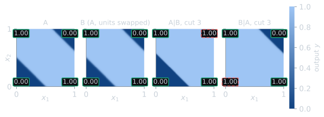
Why the cut after gene 3 fails is easiest to see from the child's genome, $[4, 4, -2, \; 4, 4, -2, \; 6, 4, -8]$. Both hidden units are OR units now, so at $(1,1)$ both are on and the output sum is $6 + 4 - 8 = 2$, which the sigmoid turns into 1, where XOR needs 0. In $A$ the NAND unit was the one that switched off at $(1,1)$, and the child inherited no copy of it. Nothing in the child's fitness can tell selection that it is one gene block away from a perfect network.
Permutation is not the only symmetry. Since $s(-z) = 1 - s(z)$, negating a hidden unit's incoming weights and bias turns its output $h$ into $1 - h$, and changing the sign of its outgoing weight $v$ and adding $v$ to the output bias restores the original function. To check the second step: the output unit receives $v h$ from the original unit, and from the negated unit it receives $-v(1 - h) + v = v h$, the same contribution. A two-hidden-unit network therefore has $2! \times 2^2 = 8$ genomes for each function, before counting near-equivalent ones. For $A$ they are, from fixed_topology_worked.py:
| Transformation of $A$ | Genome | Viable children of $A$ and it (of 16) |
|---|---|---|
| none | $[4, 4, -2, \; -3, -3, 5, \; 4, 6, -8]$ | 16 |
| negate $h_2$ | $[4, 4, -2, \; 3, 3, -5, \; 4, -6, -2]$ | 6 |
| negate $h_1$ | $[-4, -4, 2, \; -3, -3, 5, \; -4, 6, -4]$ | 0 |
| negate both | $[-4, -4, 2, \; 3, 3, -5, \; -4, -6, 2]$ | 0 |
| swap | $[-3, -3, 5, \; 4, 4, -2, \; 6, 4, -8]$ | 5 |
| swap, negate new $h_2$ | $[-3, -3, 5, \; -4, -4, 2, \; 6, -4, -4]$ | 0 |
| swap, negate new $h_1$ | $[3, 3, -5, \; 4, 4, -2, \; -6, 4, -2]$ | 4 |
| swap, negate both | $[3, 3, -5, \; -4, -4, 2, \; -6, -4, 2]$ | 4 |
All eight compute the same outputs to within $10^{-18}$, so all eight have the same fitness and selection treats them as the same network. Crossed with $A$ by one-point crossover, three of them produce no child that solves XOR at all. Negating a unit turns OR into NOR, and a child that mixes the two halves of a unit, or that takes $A$'s output weights with the other genome's hidden units, receives a signal of the wrong sign. The experiment measured how much these symmetries matter among evolved solutions. It took the 30 solutions found by the genetic algorithm with crossover and, for each of the 435 pairs, evaluated all 16 one-point children, first with the parents as evolved, then after reordering the second parent's hidden units to match the first as closely as possible (the order with the smaller squared distance between corresponding weights):
| Crossing | Children that solve XOR |
|---|---|
| Independent solutions, as evolved | 869 of 6,960 (12.5%) |
| Independent solutions, hidden units aligned | 1,120 of 6,960 (16.1%) |
| Each solution with its own permuted copy | 143 of 480 (29.8%) |
Alignment swapped the hidden units in 233 of the 435 pairs, and it raised the share of viable children by more than a quarter, from 12.5% to 16.1%. That share stays low because independent solutions also differ by sign symmetries and by the scale and pattern of their weights, which no reordering can fix. The last row isolates the permutation alone: crossing a network with a reordered copy of itself, which differs from it only in convention, still loses 70% of the children.
Inside a converged population the problem fades, because once one convention takes over, all parents share it. That is also why it matters: crossover is most useful early, when the population is diverse, and early is when the conventions compete. Some systems avoided the problem by dropping crossover altogether; Stanley and Miikkulainen (2002, §2.1.3) review examples among the methods that also evolve topology. Such et al. (2017) also left crossover out of their deep genetic algorithm, for simplicity.
Cooperative approaches: SANE and ESP
Another route evolves neurons instead of whole networks. In SANE (Symbiotic, Adaptive Neuro-Evolution), Moriarty and Miikkulainen (1996) evolved a population of hidden neurons, each a partial solution, and formed networks by combining neurons for evaluation. A neuron's fitness reflects how well the networks it takes part in perform. The authors argue that this symbiotic arrangement encourages both cooperation and specialization, which speeds the search and helps it avoid converging on poor solutions, and on the inverted pendulum task SANE built effective networks substantially faster than the Adaptive Heuristic Critic, Q-learning and the GENITOR genetic algorithm.
Enforced Sub-Populations (ESP), introduced by Gomez and Miikkulainen (1997), keeps SANE's population of neurons but splits it: there is a separate subpopulation for each of the $u$ hidden-unit positions in the network, a network is formed by drawing one neuron from each subpopulation, and a neuron recombines only with members of its own subpopulation. Gomez and Miikkulainen give two reasons this speeds up SANE. The specialized groups that have to organize themselves out of SANE's single population are fixed by design in ESP, and recombination no longer mixes neurons that fill different roles in the network. A consequence of the design, which the authors do not list among its reasons, is that a neuron's role is tied to its slot, so the reorderings behind competing conventions cannot arise between subpopulations. Gomez and Miikkulainen describe ESP's main contribution as making it possible to evolve recurrent networks, which their prey-capture task needed because the agent has to remember where it last saw the prey.
Stanley and Miikkulainen (2002, Table 1) collected published results on double pole balancing with velocity inputs, a standard control benchmark, in which two poles of different lengths on one cart must be kept upright:
| Method | Evaluations to solve (average) |
|---|---|
| Evolutionary programming (Saravanan and Fogel) | 307,200 |
| Conventional neuroevolution (Wieland) | 80,000 |
| SANE | 12,600 |
| ESP | 3,800 |
| NEAT | 3,600 |
The neuron-level methods needed 6 to 21 times fewer evaluations than conventional whole-network neuroevolution on this task, and NEAT, which also evolves the topology, matched ESP; Stanley and Miikkulainen report that the difference between NEAT and ESP was not statistically significant. On the harder variant without velocity inputs, ESP still solved the task with a fixed topology, restarting with a random number of hidden units when it became stuck, and NEAT was about five times faster. The NEAT article takes up that comparison.
When weight evolution competes with gradient descent
For supervised learning on large networks, where every example supplies a target and the loss is differentiable, backpropagation is the standard method. The comparisons below are all in reinforcement learning, where the gradient has to be estimated from rewards.
Salimans, Ho, Chen, Sidor and Sutskever (2017) used an evolution strategy to train policy networks on the MuJoCo locomotion tasks and on Atari games. Each worker perturbs the network's parameters with Gaussian noise, runs an episode and reports a single number, its return, and the updates combine the returns into an estimate of the gradient of expected return. The authors point out that this is a finite-difference derivative estimate in a randomly chosen direction. Because workers need to exchange only returns and random seeds, the method parallelized well: with 1,440 workers it solved the 3D humanoid walking task in under 10 minutes, and on Atari, with 720 CPUs and about an hour per game, it did better than published A3C results on 23 of 51 games and worse on 28.
Such, Madhavan, Conti, Lehman, Stanley and Clune (2017) asked whether an algorithm that does not estimate a gradient at all could work at that scale. Their genetic algorithm is about as simple as one can be: truncation selection of the top $T$ networks, a parent drawn uniformly from them, Gaussian noise added to every parameter, one elite copied unchanged, and no crossover. It evolved networks with over four million parameters. On Atari it was competitive overall with DQN, A3C and evolution strategies, better on some games and worse on others. It also always beat random search, but random search alone outperformed DQN on 3 of the 13 games tested, A3C on 6, and evolution strategies on 3. The authors read this as evidence that on some of these problems local optima, saddle points or noisy gradient estimates impede gradient-based methods, and that following the gradient is not always the best choice.
These results share a pattern with the small XOR experiment above. A search with no gradient can be competitive when the reward is sparse or deceptive and the space of good solutions is wide, and a random-search baseline is needed to tell whether the evolutionary machinery is doing the work. They also share the fixed topology: in both, a person chose the network and evolution chose only its weights. Evolving the structure as well is the subject of NEAT, whose historical markings were designed to make crossover between networks of different shapes meaningful, the harder form of the competing conventions problem.
References
- Gomez, F., and Miikkulainen, R. (1997). Incremental evolution of complex general behavior. Adaptive Behavior, 5(3–4), 317–342.
- Montana, D. J., and Davis, L. (1989). Training feedforward neural networks using genetic algorithms. In Proceedings of the Eleventh International Joint Conference on Artificial Intelligence (IJCAI-89), 762–767.
- Moriarty, D. E., and Miikkulainen, R. (1996). Efficient reinforcement learning through symbiotic evolution. Machine Learning, 22(1–3), 11–32.
- Radcliffe, N. J. (1993). Genetic set recombination and its application to neural network topology optimisation. Neural Computing and Applications, 1(1), 67–90.
- Salimans, T., Ho, J., Chen, X., Sidor, S., and Sutskever, I. (2017). Evolution strategies as a scalable alternative to reinforcement learning. arXiv:1703.03864.
- Schaffer, J. D., Whitley, D., and Eshelman, L. J. (1992). Combinations of genetic algorithms and neural networks: a survey of the state of the art. In COGANN-92: International Workshop on Combinations of Genetic Algorithms and Neural Networks, 1–37. IEEE.
- Stanley, K. O., and Miikkulainen, R. (2002). Evolving neural networks through augmenting topologies. Evolutionary Computation, 10(2), 99–127.
- Such, F. P., Madhavan, V., Conti, E., Lehman, J., Stanley, K. O., and Clune, J. (2017). Deep neuroevolution: genetic algorithms are a competitive alternative for training deep neural networks for reinforcement learning. arXiv:1712.06567.
- Whitley, D., Starkweather, T., and Bogart, C. (1990). Genetic algorithms and neural networks: optimizing connections and connectivity. Parallel Computing, 14(3), 347–361.
- Yao, X. (1999). Evolving artificial neural networks. Proceedings of the IEEE, 87(9), 1423–1447.