A genetic algorithm with 64 individuals evaluates each one by running a simulation that takes 20 milliseconds. Selection, crossover and mutation for the whole population take under a millisecond, so one generation costs about 1.3 seconds, nearly all of it spent waiting for fitness values. The 64 evaluations are independent of each other. Nothing about the algorithm requires them to run one after another, and a machine with 8 cores could in principle run eight at a time.
This is the idea of master-slave parallel evaluation. One process, the master, holds the population and performs selection and variation. The other processes, the slaves or workers, receive individuals, compute their fitness, and send the values back. It is the simplest way to parallelize an evolutionary algorithm, one of the oldest, and in many applications the most useful, because the expensive part of the algorithm is usually the fitness function. This article covers what master-slave evaluation changes and what it leaves alone, the model that predicts how many workers to use, and what happened when the scheme was measured on an ordinary desktop. The other way of parallelizing a genetic algorithm, dividing the population itself, is the subject of island model genetic algorithms.
Parallel implementation and parallel model
Alba and Tomassini (2002), surveying parallel evolutionary algorithms, stress the difference between an algorithm's model and its parallel implementation. The model is the algorithm as a mathematical object: how the population is structured, which individuals selection compares, which can mate. The implementation is how that algorithm is mapped onto hardware. The two choices are independent, which gives four combinations:
| Sequential implementation | Parallel implementation | |
|---|---|---|
| Panmictic model (one population, selection sees everyone) | The ordinary genetic algorithm | Master-slave evaluation |
| Structured model (subpopulations or neighbourhoods) | An island or cellular model run on one processor | An island or cellular model with one processor per deme |
Master-slave evaluation, in its synchronous form, is a parallel implementation of the panmictic model. Selection still compares every member of the population, and given the same random numbers it produces exactly the same sequence of populations as the sequential algorithm. The only thing that changes is how long each generation takes. Every theoretical result about the sequential algorithm, from takeover times to population sizing, carries over unchanged. Cantú-Paz (2000, ch. 3) makes the same point: the theory of simple genetic algorithms applies directly to choosing a master-slave algorithm's search parameters.
Structured models are different. Dividing the population into islands or placing it on a grid changes which individuals compete and mate, and therefore changes the search itself, whether or not the islands run on separate processors.
Synchronous and asynchronous schemes
The simplest master-slave algorithm is synchronous. Each generation, the master sends the new individuals to the slaves, waits until every fitness value has come back, and only then performs selection for the next generation. The generation boundary acts as a barrier. The algorithm is the sequential one, step for step, and the barrier is what guarantees that.
The barrier also costs time. If evaluation times vary, every slave that finishes early sits idle until the slowest one is done. Evaluation times vary often in practice: a simulation of a robot that falls over in the first second ends sooner than one of a robot that walks; a neural network with more connections takes longer to run; a program in genetic programming may run to its time limit.
An asynchronous master-slave algorithm removes the barrier. The master keeps every slave busy. As soon as one returns a fitness value, the master inserts that individual into the population, typically by a steady-state rule such as replacing the worst member, then creates one new child by selection and variation and sends it to the now idle slave. No slave waits for any other. In his review of early parallel genetic algorithms, Cantú-Paz (2000, ch. 3) notes that asynchronous implementations without a clear separation between generations ran faster than ones in which the master waited for the slowest slaves.
The price is that the asynchronous algorithm is a different model. It is steady-state rather than generational, and the order in which individuals enter the population depends on how long their evaluations took, which depends on the hardware, the operating system's scheduling and the other load on the machine. The run is no longer reproducible from the random seed alone. Worse, when evaluation time depends on the genotype, individuals that evaluate quickly return first and reproduce first. Scott and De Jong (2015) analyzed this scheme and found that such a bias toward fast-evaluating individuals exists in some cases. Whether it matters depends on the problem. A bias toward cheap evaluations does little harm where cheap solutions are also good ones, and it works against the search where the best solutions are the expensive ones.
Cantú-Paz's model of the optimal number of slaves
Adding slaves divides the evaluation work, but each slave also costs communication: the master must send it individuals and receive their fitness values. Cantú-Paz (2000, ch. 3) analyzed this trade-off for a synchronous algorithm with the following assumptions: the time for selection and variation is negligible, every individual takes the same time to evaluate, and every processor receives the same number of individuals. His symbols:
- $n$, the population size;
- $T_f$, the time to evaluate one individual;
- $T_c$, the time the master spends communicating with one slave in a generation;
- $P$, the number of processors. The master also evaluates a share, so there are $S = P - 1$ slaves.
Communication with the slaves costs $P\,T_c$ per generation, while every processor evaluates its $n/P$ individuals. The elapsed time of one generation is then
$$T_p = P\,T_c + \frac{n\,T_f}{P}.$$
The first term grows with $P$ and the second shrinks, so there is a best number of processors. The derivation takes four short steps.
- Differentiate. Treating $P$ as continuous, $\dfrac{dT_p}{dP} = T_c - \dfrac{n\,T_f}{P^2}$. The first part is the extra communication one more processor costs; the second is the evaluation time it saves, which shrinks as $1/P^2$ because each new processor takes a smaller share.
- Set the derivative to zero. The two effects balance where $T_c = n\,T_f / P^2$, that is, where $P^2 = n\,T_f / T_c$.
- Check that it is a minimum. The second derivative, $2\,n\,T_f / P^3$, is positive for every $P > 0$, so $T_p$ is convex in $P$ and the stationary point is its only minimum.
- Name the ratio. Writing $\gamma = T_f / T_c$ for the ratio of evaluation time to communication time,
$$P^* = \sqrt{\frac{n\,T_f}{T_c}} = \sqrt{\gamma\, n},$$
and the optimal number of slaves is $S^* = P^* - 1$. The ratio $\gamma$ does most of the work. A cheap fitness function on a slow network has small $\gamma$ and gains little from parallelism; an expensive simulation has large $\gamma$ and can use many processors. The square root matters too: quadrupling the population or the cost of an evaluation only doubles the number of processors worth using.
Substituting $P^*$ back into the two terms of $T_p$ gives $P^* T_c = \sqrt{n\,T_f\,T_c}$ and $n\,T_f / P^* = \sqrt{n\,T_f\,T_c}$: at the optimum, communication and evaluation take exactly the same time. The sequential generation takes $T_s = n\,T_f$, so the best possible speedup is
$$\frac{T_s}{T_p} = \frac{n\,T_f}{2\sqrt{n\,T_f\,T_c}} = \frac{1}{2}\sqrt{\frac{n\,T_f}{T_c}} = \frac{P^*}{2}.$$
The efficiency, speedup divided by the number of processors, has a closed form at every $P$. Dividing numerator and denominator of $T_s / (P\,T_p)$ by $n\,T_f$,
$$E(P) = \frac{n\,T_f}{P^2 T_c + n\,T_f} = \frac{1}{1 + P^2 / (\gamma\, n)} = \frac{1}{1 + (P/P^*)^2}.$$
Efficiency depends only on how $P$ compares with $P^*$. It is 99% at $P = P^*/10$, 80% at $P^*/2$, and exactly 50% at $P^*$: at its optimal configuration a master-slave algorithm spends half its time communicating. The optimum minimizes the time per generation, not the cost in processor-hours, and a user paying for processors would stop well short of it.
Cantú-Paz also derives the condition for parallelism to help at all. The smallest parallel configuration, $P = 2$, is faster than the sequential algorithm when $2\,T_c + n\,T_f/2 < n\,T_f$. Subtracting $n\,T_f/2$ from both sides gives $2\,T_c < n\,T_f / 2$, which is $\gamma > 4/n$. With a population of 64, evaluation must cost more than a sixteenth of a message. He argues too that a more detailed communication cost, with a bandwidth term proportional to the size of the message and a fixed latency per message, changes $P^*$ little in most cases, because latency dominates.
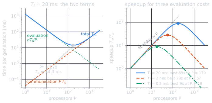
A worked example. With $n = 64$, $T_f = 20$ ms and $T_c = 0.04$ ms, $\gamma = 500$ and $P^* = \sqrt{64 \times 20 / 0.04} = \sqrt{32{,}000} \approx 179$, and the best speedup is about 89. The sequential generation takes $T_s = 64 \times 20 = 1{,}280$ ms. The model's prediction at a range of processor counts (computed by tools/experiments/evolution/master_slave_model.py, rounded to two decimals):
| $P$ | Communication $P\,T_c$ (ms) | Evaluation $n\,T_f/P$ (ms) | $T_p$ (ms) | Speedup | Efficiency |
|---|---|---|---|---|---|
| 2 | 0.08 | 640.00 | 640.08 | 2.00 | 1.00 |
| 16 | 0.64 | 80.00 | 80.64 | 15.87 | 0.99 |
| 64 | 2.56 | 20.00 | 22.56 | 56.74 | 0.89 |
| 128 | 5.12 | 10.00 | 15.12 | 84.66 | 0.66 |
| 179 | 7.16 | 7.15 | 14.31 | 89.44 | 0.50 |
| 256 | 10.24 | 5.00 | 15.24 | 83.99 | 0.33 |
| 512 | 20.48 | 2.50 | 22.98 | 55.70 | 0.11 |
At $P = 16$ the prediction is nearly linear: $T_p = 0.64 + 80 = 80.64$ ms, a speedup of $1280 / 80.64 \approx 15.9$. Past the optimum the curve turns over, and 512 processors are slower than 64. With $T_f = 2$ ms, $P^* \approx 57$ and the best speedup is about 28; with $T_f = 0.2$ ms, $P^* \approx 18$ and the best speedup about 9.
Amdahl's law
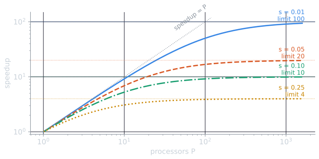
Cantú-Paz's model ignores the master's own work. Amdahl (1967) argued that the part of a computation that cannot be parallelized limits the benefit of adding processors, however many there are. The usual form of the argument is short. Let a computation take time $T$ on one processor, and let a fraction $s$ of that time be inherently serial. On $P$ processors the serial part still takes $sT$, while the rest, if it divides perfectly, takes $(1 - s)T/P$. The speedup is the ratio of the two running times, and $T$ cancels:
$$\text{speedup}(P) = \frac{T}{sT + (1 - s)T/P} = \frac{1}{s + (1 - s)/P} \le \frac{1}{s}.$$
The bound is reached only as $P \to \infty$, and the approach is slow. Setting the speedup to half its limit, $1/(2s)$, requires $s + (1 - s)/P = 2s$, so $P = (1 - s)/s$: with $s = 0.05$, 19 processors reach half the limit of 20, and every further gain costs more processors than the last. With $s = 0.05$, 16 processors give a speedup of $1/(0.05 + 0.95/16) \approx 9.1$, and no number of processors gives more than 20.
In a master-slave genetic algorithm the serial part is selection, variation, bookkeeping, and the fixed cost of each round of messages, all performed by the master while the slaves wait. In the measurement below with $T_f = 0.19$ ms, the 1.14 ms fixed cost per parallel generation was 9% of the sequential generation, which by itself caps the speedup near $1/0.09 \approx 11$. Amdahl's bound ignores communication, though: in Cantú-Paz's model the time per generation starts rising again well before Amdahl's curve has flattened. The two views agree on the practical conclusion: master-slave evaluation pays when evaluation dominates the generation, and pays more the more it dominates.
Measured on a desktop
The script tools/experiments/evolution/master_slave.py in the site repository runs a genetic algorithm on OneMax (64 bits, population 64, binary tournament, uniform crossover, bit-flip mutation at rate 1/64) whose fitness function also performs a fixed number of iterations of a pure-Python arithmetic loop. The number of iterations is calibrated so that one evaluation costs a chosen $T_f$ on one core. The workers are processes from Python's multiprocessing module, and each generation the master sends each worker one batch of $\lceil n/S \rceil$ individuals. Here the master only waits, so the number of workers $S$ plays the role of Cantú-Paz's $P$. The machine has an Intel Core i9-9900K with 8 cores and 16 hardware threads, and one other single-threaded job (another experiment) was running during the measurements. Times are the fastest of five repetitions.
Communication cost. With $T_f \approx 0$, a parallel generation took between 1.12 ms ($S = 1$) and 1.80 ms ($S = 16$). A least-squares line through the six measurements gives a fixed cost of $T_0 = 1.14$ ms per generation and $T_c = 0.045$ ms per worker. Interprocess communication on one machine is cheap. The fixed cost is not: it exceeds the 0.88 ms the whole sequential generation takes with free evaluations.
Speedup. With $T_f = 20.2$ ms, the measured sequential generation took 1,293 ms. The model's prediction, $T_0 + n\,T_f/S + S\,T_c$ with the measured constants, gives $S^* = 170$ and a best speedup of 79:
| Workers $S$ | Measured $T_p$ (ms) | Speedup | Model $T_p$ (ms) | Model speedup | Time per evaluation in a worker (ms) |
|---|---|---|---|---|---|
| 1 | 1,353 | 0.96 | 1,293 | 1.00 | 21.1 |
| 2 | 687 | 1.88 | 647 | 2.00 | 21.3 |
| 4 | 386 | 3.35 | 324 | 3.99 | 22.8 |
| 8 | 280 | 4.61 | 163 | 7.93 | 29.7 |
| 12 | 252 | 5.14 | 109 | 11.82 | 36.5 |
| 16 | 239 | 5.41 | 83 | 15.65 | 50.8 |
Up to four workers the model holds to within about 20% (386 ms measured against 324 ms predicted). Beyond that it fails, and the last column shows why. The model treats $T_f$ as a constant of the problem, but the time one evaluation took inside a worker rose from 21.1 ms with one worker to 29.7 ms with eight and 50.8 ms with sixteen. Communication was not the bottleneck: the script also records the total evaluation time of the busiest worker in each generation, and it came within 1% of $T_p$ in every row up to twelve workers and within 7% with sixteen, so almost all of each generation was spent evaluating. Sixteen workers on 8 physical cores share each core between two hardware threads, and another program was competing for the same cores; even eight workers could not each have a core to themselves. On this machine, eight workers bought a speedup of 4.6, and doubling to sixteen added less than one more.
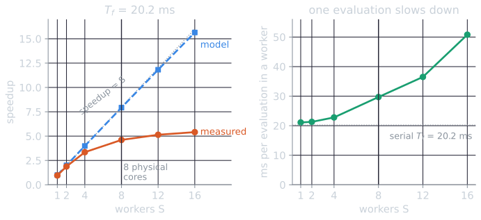
The row for one worker also shows what a fair baseline is. A single worker was about 5% slower than the sequential program (1,353 ms against 1,293, a speedup of 0.96), because it adds the cost of sending the population to another process and back without dividing any work. Speedups measured against the parallel program run with one worker, rather than against the best sequential program, look better than they are.
Cheaper evaluations fared worse, as the model predicts, though for a different reason than it gives. With $T_f = 2.0$ ms the speedup was 3.42 with four workers and 4.53 with sixteen (the model predicted 3.87 and 13.06). With $T_f = 0.19$ ms it peaked at 3.17 with sixteen workers, against a predicted 5.05; here the 1.14 ms fixed cost per generation, which Amdahl's law treats as serial work, is already 9% of the sequential generation time. In every configuration the final population's best fitness was identical to the sequential run's, as it must be: the parallel implementation did not change the algorithm.
The general lesson is that $T_f$ and $T_c$ should be measured on the hardware that will run the algorithm, under the load it will actually carry, and with as many workers as will be used. The earlier document similarity experiment in the information retrieval part of this site met the same limit from the other side: when each task is cheap, the fixed cost of starting and feeding worker processes outweighs the work they share.
Uneven evaluation times
Where the barrier loses time
A small schedule shows the mechanism before any measurement. Four workers evaluate three generations of eight individuals, 24 evaluations whose costs are drawn from $5\,\text{ms} \times m$ with $m$ uniform on $[0.1, 1.9]$, so they range from about 0.5 ms to 9.3 ms. The schedule is computed in virtual time by tools/experiments/evolution/master_slave_model.py, with no communication cost at all, so the barrier is the only difference between the two schemes. In the synchronous scheme each evaluation goes to the first idle worker, and the next generation cannot start until the slowest evaluation of the current one is done. In the first generation the last evaluation finishes at 7.71 ms, while worker 1 has been idle since 7.02 ms; in the second generation, worker 3 sits idle from 17.51 ms to 22.72 ms waiting for worker 2. The asynchronous scheme hands out the next evaluation the moment a worker frees up.
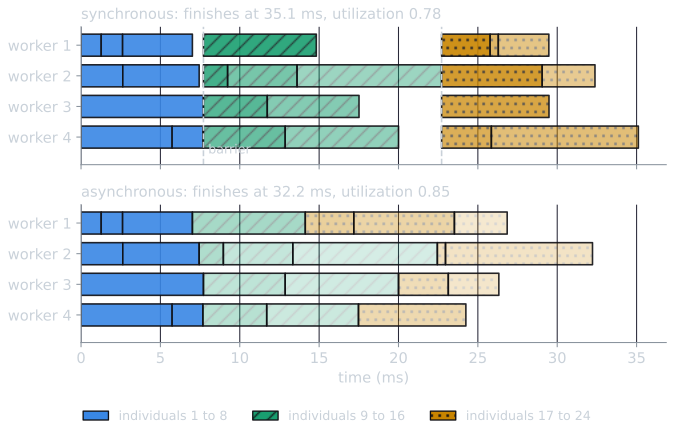
The total work is 109.6 ms, so four perfectly busy workers would need 27.4 ms. The synchronous schedule takes 35.1 ms (utilization 0.78) and the asynchronous one 32.2 ms (0.85). The asynchronous scheme is not free of idle time either: the last evaluations to start determine when the run ends, and here a 9.3 ms evaluation began at 22.96 ms. Over a long run this end effect is paid once, while the synchronous scheme pays its barrier every generation.
How much the barrier costs depends on two things: how variable the evaluation times are, and how many evaluations each worker performs per generation. With more evaluations per worker, the uneven loads average out before the barrier. Simulating 640 evaluations on 8 workers in the same way, over 30 seeds (medians, interquartile ranges within 0.01 of them):
| Evaluations per generation | Spread of $m$ | Synchronous utilization | Asynchronous utilization | Asynchronous time / synchronous time |
|---|---|---|---|---|
| 16 | none ($m = 1$) | 1.000 | 1.000 | 1.000 |
| 16 | $[0.7, 1.3]$ | 0.854 | 0.994 | 0.859 |
| 16 | $[0.4, 1.6]$ | 0.767 | 0.992 | 0.772 |
| 16 | $[0.1, 1.9]$ | 0.725 | 0.990 | 0.733 |
| 8 | $[0.1, 1.9]$ | 0.591 | 0.990 | 0.597 |
| 32 | $[0.1, 1.9]$ | 0.844 | 0.990 | 0.852 |
| 64 | $[0.1, 1.9]$ | 0.917 | 0.990 | 0.925 |
With equal evaluation times the barrier costs nothing. With one evaluation per worker per generation and costs spread over $[0.1, 1.9]$, the synchronous scheme wastes 41% of the workers' time, because every generation lasts as long as its slowest evaluation. With eight evaluations per worker the waste falls to 8%.
Measured
The third part of the script gives each evaluation a cost of $5\,\text{ms} \times m$, with $m$ drawn uniformly from $[0.1, 1.9]$, and runs 640 evaluations on 8 workers with a population of 16, in two ways. The synchronous version submits each generation's 16 evaluations together, letting an idle worker take the next waiting task, and waits for all of them. The asynchronous version keeps 8 evaluations in flight and, as each finishes, inserts the result by replacing the worst member if it is better and submits one new child. Over five alternating repetitions (medians):
| Scheme | Wall time | Utilization of the 8 workers |
|---|---|---|
| Synchronous | 0.854 s | 0.47 |
| Asynchronous | 0.627 s | 0.63 |
The total evaluation work was about 3.2 seconds in both cases, and the asynchronous scheme finished it in 73% of the synchronous time (median of the paired ratios). Neither approaches full utilization, because of the same per-message overhead and shared cores as before, but removing the barrier recovered a large part of the idle time. The ratio of wall times, 0.73, is close to the 0.733 that the zero-overhead simulation predicts for the same configuration (16 evaluations per generation on 8 workers, $m$ in $[0.1, 1.9]$). Read together, the two suggest that the per-message overhead and the shared cores slowed both schemes by a similar factor, and that the difference between them is the barrier. The comparison measures throughput only. The two schemes are different algorithms, a generational one and a steady-state one, so the populations they produce differ, and the right choice depends on whether the evaluations or the search dynamics matter more.
Clusters and accelerators
The same design scales from cores to machines, with $T_c$ now a network round trip and $T_f$ often a full simulation. Its weak point at large scale is the master, which must send every genome and receive every fitness value. Salimans, Ho, Chen, Sidor, and Sutskever (2017) removed most of that traffic for an evolution strategy that trains neural network policies. Every worker knows the random seeds of all the others, so each can reconstruct every perturbation of the parameters itself, and the workers need to exchange only scalar returns. They report scaling to over a thousand parallel workers and solving 3D humanoid walking in 10 minutes.
On graphics processors and other accelerators the picture changes again. When the fitness function can be written as array operations, the whole population can be evaluated as one batch, and the master-slave distinction collapses into vectorization. Libraries such as evosax (Lange, 2023) implement evolution strategies and genetic algorithms in JAX, so that the search itself runs on the accelerator alongside a fitness function written in the same framework. This works only when the evaluation itself can be expressed in that form; a fitness function that calls an external simulator remains a task for a pool of conventional workers.
Common misreadings
- "More workers are always at least as fast." In Cantú-Paz's model, past $P^*$ every extra processor adds more communication than it removes evaluation, and in the measurement above sixteen workers on eight cores made each evaluation two and a half times slower.
- "Parallel evaluation changes the search." The synchronous scheme does not: given the same seed it produces the same populations. Only the asynchronous scheme, which is a steady-state algorithm with an order of insertion set by the hardware, changes what the algorithm does.
- "The model's $T_f$ is the time one evaluation takes." It is the time one evaluation takes on the processors and under the load the parallel run actually has, which the measurement showed can be more than double the single-core figure.
- "Efficiency of 50% at the optimum means something is wrong." It is what the model predicts at $P^*$. A run that should be economical with processors belongs well below $P^*$, where efficiency is close to 1.
When it pays
Master-slave evaluation is worth using when evaluation dominates the generation time and the evaluations are independent. It requires no change to the algorithm's design, and in its synchronous form it keeps every property of the sequential algorithm, including reproducibility. Its benefit is bounded by the serial work the master does, by the cost of communicating with each slave, and, as the measurement above showed, by how the slaves share the hardware. The asynchronous form trades reproducibility and the generational model for higher utilization when evaluation times vary. When more processors are available than one population can use, or when the goal is a different search rather than a faster one, the population itself can be divided, which is the subject of island models.
References
- Alba, E., and Tomassini, M. (2002). Parallelism and evolutionary algorithms. IEEE Transactions on Evolutionary Computation, 6(5), 443–462.
- Amdahl, G. M. (1967). Validity of the single processor approach to achieving large scale computing capabilities. In Proceedings of the AFIPS Spring Joint Computer Conference, 30, 483–485.
- Cantú-Paz, E. (2000). Efficient and Accurate Parallel Genetic Algorithms, chapter 3. Kluwer Academic Publishers.
- Lange, R. T. (2023). evosax: JAX-based evolution strategies. In Proceedings of the Companion Conference on Genetic and Evolutionary Computation (GECCO '23 Companion), 659–662.
- Salimans, T., Ho, J., Chen, X., Sidor, S., and Sutskever, I. (2017). Evolution strategies as a scalable alternative to reinforcement learning. arXiv:1703.03864.
- Scott, E. O., and De Jong, K. A. (2015). Understanding simple asynchronous evolutionary algorithms. In Proceedings of the 2015 ACM Conference on Foundations of Genetic Algorithms XIII, 85–98.