Evolving only the weights of a fixed network leaves a person to choose the network: how many hidden units, which connections. Letting evolution choose the structure too sounds like a straightforward extension, and many systems tried it in the 1990s. Stanley and Miikkulainen (2002) identified three questions that such a system must answer. Is there a genetic representation that lets networks of different shapes cross over in a meaningful way? How can a new piece of structure, which usually lowers fitness until its weights are tuned, survive long enough to be tuned? And how can networks be kept small without adding a penalty for size to the fitness function? NeuroEvolution of Augmenting Topologies (NEAT) is their answer to all three, and its three components, historical markings, speciation and growth from minimal structure, map onto the three questions.
This article follows the paper (Stanley and Miikkulainen, 2002), works its crossover example by hand, checks the reported results against the paper's tables, and reports a reimplementation, tools/experiments/evolution/neat.py in the site repository, run on the paper's XOR task.
The genome
A NEAT genome has two lists. Node genes name the network's inputs, outputs and hidden units. Connection genes each specify an in-node, an out-node, a weight, an enable bit, and an innovation number. A disabled connection gene stays in the genome but is not expressed in the network. The genome for a network with three inputs (nodes 1 to 3), one output (node 4) and one hidden unit (node 5) might read:
| Innovation | 1 | 2 | 3 | 4 | 5 | 6 |
|---|---|---|---|---|---|---|
| Connection | 1→4 | 2→4 | 3→4 | 2→5 | 5→4 | 1→5 |
| Enabled | yes | no | yes | yes | yes | yes |
The network it expresses has the direct connections from inputs 1 and 3 to the output, and paths from inputs 1 and 2 through hidden node 5. The disabled gene 2→4 records a connection that a mutation split.
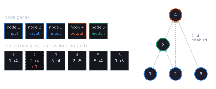
Unlike the fixed-topology genome, where position 7 always means the same weight, a NEAT genome has no fixed positions. Its length changes as the network grows, and two genomes of the same length can describe different networks. What gives a gene its identity is its innovation number, described below.
Mutation changes weights, as in any neuroevolution system, and it changes structure in two ways:
- Add connection. A new connection gene with a random weight joins two previously unconnected nodes.
- Add node. An existing connection is split: the old gene is disabled, a new node is placed where the connection was, and two new connection genes are added. The connection into the new node gets weight 1 and the connection out of it gets the old connection's weight.
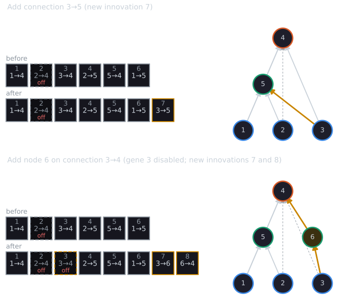
The add-node rule is chosen to change the network's function as little as possible. The new node does add a nonlinearity, so the function changes slightly, but the node is connected and working from the start, rather than being dead structure that would have to be wired in later.
How much an added node changes the function
"Slightly" depends on the activation function and on the signals involved, and a small example shows how much. Take a minimal XOR genome, the starting point of every run below: inputs $x_1$ and $x_2$, a bias input fixed at 1, and one output, with weights 2 from each input and $-1$ from the bias. Through the steepened sigmoid $s(z) = 1/(1 + e^{-4.9z})$ it computes OR. Splitting its connection from $x_1$ disables that gene and routes $x_1$ through a new hidden node $h = s(1 \cdot x_1)$, whose output reaches the output unit with the old weight 2. The values, from tools/experiments/evolution/neat_worked.py (Part 1), rounded to four decimals:
| $x_1$ | $x_2$ | output before | $h = s(x_1)$ | output after |
|---|---|---|---|---|
| 0 | 0 | 0.0074 | 0.5000 | 0.5000 |
| 0 | 1 | 0.9926 | 0.5000 | 0.9999 |
| 1 | 0 | 0.9926 | 0.9926 | 0.9921 |
| 1 | 1 | 1.0000 | 0.9926 | 1.0000 |
Where $x_1 = 1$ the new path passes almost the same signal as the old connection, since $s(1) = 0.9926$, and the outputs barely move. Where $x_1 = 0$ the old connection carried $2 \times 0 = 0$, but the new node outputs $s(0) = 0.5$, so the path now carries $2 \times 0.5 = 1$, and the output for $(0, 0)$ jumps from 0.0074 to 0.5. The fitness falls from 8.8674 to 6.2101. The rule would preserve the function exactly only if the new node passed its input through unchanged, which a sigmoid centred at zero never does. This is the cost that the next section's markings cannot remove and that speciation exists to absorb: the mutated network is worse than its parent until its new weights are tuned, here by a bias into the new node or a change in the weights around it.
Historical markings
When networks of different shapes mate, which gene in one corresponds to which gene in the other? Matching by structure is expensive and ambiguous, which is the topology-level form of the competing conventions problem. NEAT's answer is that two genes with the same historical origin represent the same structure, even if their weights differ, because both descend from one ancestral gene. So NEAT records the origin. Whenever a structural mutation creates a new gene, a global counter is incremented and its value becomes the gene's innovation number. Genes keep their numbers forever, through every crossover.
One refinement prevents an explosion of numbers. If the same structural mutation occurs in several genomes in the same generation, for example two networks both adding the connection 3→5, each would otherwise get a different number. NEAT keeps a list of the innovations made in the current generation, and identical mutations within one generation receive the same number.
Crossover by innovation number
Lining two genomes up by innovation number sorts their genes into three kinds. Matching genes have the same number in both parents. Genes that do not match are disjoint if their number falls within the range of the other parent's numbers, and excess if it lies beyond the other parent's largest number. The child inherits each matching gene from a randomly chosen parent, and inherits all disjoint and excess genes from the fitter parent. A gene disabled in either parent has a preset chance of being disabled in the child, 75% in the paper's experiments.
The paper's Figure 4 crosses these two parents. Nodes 1 to 3 are inputs, 4 the output, 5 and 6 hidden:
| Innovation | 1 | 2 | 3 | 4 | 5 | 6 | 7 | 8 | 9 | 10 |
|---|---|---|---|---|---|---|---|---|---|---|
| Parent 1 | 1→4 | 2→4 off | 3→4 | 2→5 | 5→4 | 1→5 | ||||
| Parent 2 | 1→4 | 2→4 off | 3→4 | 2→5 | 5→4 off | 5→6 | 6→4 | 3→5 | 1→6 | |
| Kind | match | match | match | match | match | disjoint | disjoint | disjoint | excess | excess |
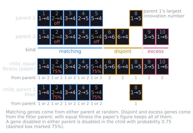
Parent 1's largest number is 8. Genes 1 to 5 match. Genes 6 and 7, present only in parent 2, and gene 8, present only in parent 1, lie within both parents' ranges and are disjoint. Genes 9 and 10 lie beyond parent 1's largest number and are excess. In parent 2, gene 5 (5→4) is disabled and genes 6 and 7 route the same path through a new node 6: the trace of an add-node mutation. Both lineages also added connections of their own (gene 8 in parent 1, genes 9 and 10 in parent 2).
In the figure the parents are equally fit, and the caption states that in that case disjoint and excess genes are also inherited at random; the offspring shown has all ten genes. Without any analysis of the networks' shapes, the child combines the structure the parents share with the structure each added. The reimplementation (tools/experiments/evolution/neat_xor.py, Part 1) follows the same rules but, for equal fitness, includes each disjoint or excess gene with probability 0.5 rather than all of them. With numpy seed 0 the equal-fitness child received genes 1 to 5 and, of the five unmatched genes, only gene 10 (1→6); its gene 5 came out disabled, as the 75% rule makes likely when one parent has it disabled. When parent 1 is made the fitter, the child takes genes 1 to 5 from either parent and, among the rest, only parent 1's gene 8 (1→5), so it has parent 1's shape. A child built with gene 10 but without genes 6 and 7 contains a connection to node 6 with no path out of it; such dangling structure is harmless in a feed-forward evaluation and can be connected later by mutation.
Alignment by innovation number costs one merge of two sorted lists, linear in the genomes' lengths, and needs no comparison of network shapes at all. It also degrades gracefully: two genomes that share no history line up as nothing but disjoint and excess genes, and crossover then hands the child the fitter parent's structure intact, rather than a mixture of unrelated parts.
The demo treats every mutation as happening in the same generation, so the same structural mutation made in both parents receives the same innovation number, the rule described under historical markings. Mutating both parents in the same way and then crossing them shows the point of that rule: the shared new genes count as matching, not as two disjoint genes.
Speciation, in brief
A network that has just gained a node usually performs worse than its parent until the new weights are tuned, and in a population where everything competes with everything, it tends to be removed before that happens. NEAT protects such innovations by dividing the population into species, so that a network competes mainly with similar networks. Historical markings make similarity cheap to measure. The compatibility distance between two genomes is
$$\delta = \frac{c_1 E}{N} + \frac{c_2 D}{N} + c_3 \bar{W},$$
where $E$ and $D$ are the numbers of excess and disjoint genes, $\bar{W}$ is the average weight difference of matching genes (disabled genes included), and $N$ is the number of genes in the larger genome, which can be set to 1 when both genomes have fewer than 20 genes. The paper's experiments used $c_1 = c_2 = 1.0$ and $c_3 = 0.4$, and a genome joins the first species whose representative is within the threshold $\delta_t = 3.0$. These are the settings for XOR and the smaller pole-balancing tasks; for the hardest task, with a population of 1,000, the paper used $c_3 = 3.0$ and $\delta_t = 4.0$. They are the paper's experimental settings, not universal constants.
For the Figure 4 parents, $E = 2$, $D = 3$ and $N = 1$, so even with identical weights on the matching genes $\delta = 2 + 3 = 5$, above $\delta_t = 3$: the two parents would sit in different species. Within species, NEAT uses explicit fitness sharing (Goldberg and Richardson, 1987): each network's fitness is divided by the size of its species, and each species receives offspring in proportion to its summed shared fitness, so no single species can take over the population. Species whose best fitness has not improved for 15 generations stop reproducing. The details, and what happens without them, are in speciation in NEAT; fitness sharing itself is described with the other niching methods.
Starting minimally
Many earlier systems that evolved topology started from random networks, which gives structural diversity from the first generation. Stanley and Miikkulainen argue that it also fills the population with nodes and connections that no evaluation has justified, so the search runs in more dimensions than the problem needs, and nothing in recombination pushes the networks back toward small ones. Some systems penalized size in the fitness function, but, as the paper notes, how large the penalty should be is hard to know, and it changes the problem being solved.
NEAT instead starts every genome with no hidden nodes, the inputs connected directly to the outputs, and adds structure only by mutation. Structure that does not help is not selected, so networks grow only as far as fitness rewards. The paper argues that this keeps the dimension of the weight space small throughout the run, not just at the end, and that this, more than the size of the final network, is where the speed comes from. Starting minimally depends on speciation: without protection, the first structural mutations would not survive, and the population would stay at its minimal form. The process of growing structure over generations is often called complexification. A comparable concern arises in genetic programming, where trees tend to grow without improving fitness.
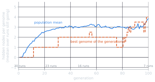
The figure shows complexification on XOR with the reimplementation described below. Taking the median over the runs still going, the population's mean number of hidden nodes per genome was 1.41 at generation 10, 2.71 at generation 25 and 3.06 at generation 50, and its mean number of enabled connections grew from the initial 3 to 6.17, 9.65 and 11.89 at the same generations (neat_worked.py, Part 2). The best network of each generation lagged behind: its median number of hidden nodes was still 0 at generation 10 and reached 1 by generation 25. Structure appears in the population first, and only some of it becomes part of the best network once its weights are tuned, which is the sequence speciation is meant to allow. The rise after generation 80 belongs to the few slow runs, which keep adding structure while they wait on the plateau described in the reimplementation section.
What the paper reports
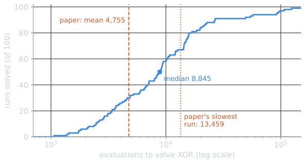
XOR. XOR cannot be computed without a hidden unit, so it tests whether NEAT can grow the structure it needs. Every initial genome connected the two inputs and a bias input, fixed at 1.0, directly to the output with random weights. Fitness was the summed absolute error on the four patterns, subtracted from 4 and squared. Every node used the steepened sigmoid $1 / (1 + e^{-4.9x})$. Over 100 runs, NEAT found a solution in an average of 32 generations and 4,755 network evaluations (standard deviation 2,553). The average solution had 2.35 hidden nodes (standard deviation 1.11) and 7.48 enabled connections, and the smallest possible solution, with one hidden node, was found in 22 runs. No run failed, and the slowest took 13,459 evaluations. The paper does not state what counted as a solution.
Pole balancing. On balancing two poles with velocity inputs, NEAT needed an average of 3,600 evaluations over 120 runs, against 3,800 for ESP, a difference the authors report as not statistically significant; NEAT's solutions used 0 to 4 hidden nodes, where the fixed-topology methods used 10. Without velocity inputs, which requires recurrent connections to estimate the missing velocities, NEAT averaged 33,184 evaluations over 20 runs, against 169,466 for ESP and 840,000 for Gruau et al.'s Cellular Encoding, with no significant difference in how well the solutions generalized.
Ablations. The paper removed one component at a time on the pole-balancing task with velocities, with up to 1,000 generations per run. Averages exclude failed runs:
| Variant | Evaluations (average) | Failure rate |
|---|---|---|
| No growth (fixed topology, 10 hidden units) | 30,239 | 80% |
| Nonspeciated (random initial topologies) | 25,600 | 25% |
| Initial random topologies | 23,033 | 5% |
| Nonmating (mutation only) | 5,557 | 0% |
| Full NEAT | 3,600 | 0% |
Each ablated version was significantly worse than full NEAT. Two details matter for reading the table. The no-growth variant was given a fully connected hidden layer of 10 units, as fixed-topology methods use on this task, since a NEAT that could not grow would otherwise have no hidden units at all. And the nonspeciated variant had to start from random topologies, because without speciation no new structure would survive from a minimal start; the authors observed that its population converged within about 10 generations on whichever topology happened to do best at first, on average one with about 5 hidden nodes. Historical markings were not ablated, because speciation and crossover both depend on them.
A reimplementation on XOR
The reimplementation uses every setting the paper gives: a population of 150; $c_1 = c_2 = 1.0$, $c_3 = 0.4$, $\delta_t = 3.0$; no reproduction for species stagnant 15 generations; species champions copied unchanged in species of more than five; an 80% chance of weight mutation, in which each weight is perturbed (90%) or replaced (10%); a 75% chance of disabling an inherited gene that was disabled in either parent; 25% of offspring by mutation alone; an interspecies mating rate of 0.001; add-node and add-connection probabilities of 0.03 and 0.05; the steepened sigmoid; and the rule from the paper's footnote that if the whole population fails to improve for more than 20 generations, only the top two species reproduce.
The paper leaves other details open, and each choice made here is documented in the module: initial and replacement weights uniform in $[-2, 2]$; perturbations uniform in $[-0.5, 0.5]$; the top 20% of each species as parents; offspring of crossover mutated too; and a network counted as solving XOR when every output is on the correct side of 0.5. One choice departs from the paper, whose stagnation rule has no exception: the species holding the current champion is exempt from it. A run stops at the first network that solves XOR and counts evaluations up to and including it, with a limit of 1,000 generations. Over 100 seeds, with median and interquartile range (Q1 to Q3) alongside the mean:
| Measure | Paper (100 runs, mean) | Reimplementation (100 seeds): median [Q1, Q3] | Reimplementation: mean (sd) |
|---|---|---|---|
| Evaluations to solve | 4,755 (sd 2,553) | 8,845 [3,912, 15,026] | 15,286 (22,757) |
| Generations | 32 | 59 [26.5, 101] | 102.4 (151.7) |
| Hidden nodes in the solution | 2.35 (sd 1.11) | 4 [2, 5] | 4.23 (3.13) |
| Enabled connections | 7.48 | 13 [10, 17] | 13.30 (4.45) |
| One-hidden-node solutions | 22 of 100 | 16 of 99 | |
| Failures | 0 of 100 | 1 of 100 (1,000 generations) | |
| Slowest successful run | 13,459 evaluations | 123,972 evaluations |
The first 30 seeds alone give a median of 8,348 evaluations [3,657, 14,587], 4 hidden nodes [2, 4] and no failures, close to the full 100.
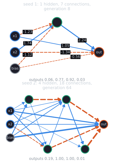
The seed 1 network is worth reading. Its hidden node computes $s(-1.23 x_1 + 1.74 x_2 - 1.12)$, which is near 1 only for the input $(0, 1)$, and the output adds $2.24$ times that to $1.05 x_1 - 1.34 x_2 - 0.56$. On $(1, 0)$ the direct path alone gives $1.05 - 0.56 = 0.49$, so the output is 0.92. On $(0, 1)$ the direct path is negative, $-1.34 - 0.56 = -1.90$, and the hidden node must make up the difference, which leaves the output at only 0.77. The network solves XOR by the paper's criterion, every output on the correct side of 0.5, with margins that further weight tuning would widen; it is not the clean OR-and-NAND construction a person would write.
The reimplementation does what the paper says NEAT does: starting from networks with no hidden units, it grew the hidden structure that XOR requires in 99 of 100 runs, and in 16 runs it found the minimal one-hidden-node solution. It did so less efficiently than the paper reports. Its median run took about twice the paper's mean number of evaluations, its mean was about three times the paper's, and its solutions were larger, with 4.23 hidden nodes on average against 2.35. The distribution has a long right tail that the paper's runs did not show: the slowest of our 99 successes took 123,972 evaluations, against the paper's worst of 13,459, and one run did not finish within 1,000 generations.
Our diagnosis of the slow runs is a fitness trap. A network whose saturated outputs are right on three patterns and wrong on the fourth scores exactly 9 out of 16, and the initial networks, with no hidden units, can reach that score by weight changes alone, for example by computing OR. The runs slower than the median spent a median of 90.5 generations with their best network scoring within 0.01 of 9, against 17 for the faster half. In our reading, a slow run is mostly time spent on that plateau until some hidden node survives long enough to have its weights tuned. The same trap stopped 6 of 30 mutation-only runs of the fixed-network genetic algorithm in evolving neural network weights. Why the paper's runs escaped it more reliably cannot be settled from the paper, because the details that govern this behavior, the size of weight perturbations, the weight range, how many members of each species reproduce, and the test for a solution, are not given.
Part 4 of neat_xor.py varies these choices one at a time, 30 seeds each with a 300-generation limit, against the default's median of 7,123 evaluations and 3 runs unfinished at that limit:
| Change | Evaluations, median [Q1, Q3] | Unfinished at 300 generations |
|---|---|---|
| None (default) | 7,123 [3,519, 13,158] | 3 |
| Initial weights in $[-1, 1]$ | 10,207 [5,029, 14,348] | 3 |
| Perturbation in $[-1, 1]$ | 7,812 [3,403, 10,628] | 2 |
| Gaussian perturbation, sd 0.5 | 6,910 [3,960, 13,626] | 4 |
| Weights clamped to $[-3, 3]$ | 6,180 [3,513, 9,564] | 0 |
| Weights clamped to $[-4, 4]$ | 10,196 [4,915, 12,776] | 1 |
| Weights clamped to $[-8, 8]$ | 8,720 [3,656, 12,900] | 0 |
| Top 50% of each species reproduce | 6,501 [3,270, 11,646] | 2 |
| Structural and weight mutations mutually exclusive | 10,127 [7,841, 16,534] | 7 |
No single change brought the median near the paper's mean of 4,755, so the gap likely comes from a combination of choices or from details of the original code that the paper does not describe. Turning off the footnote rule, which lets only the two best species reproduce after more than 20 generations without progress, left 2 of 30 runs unsolved at 1,000 generations, against none with it.
XOR versions of the ablations
The paper's ablations were run on pole balancing, a task where the right structure is not known in advance. Running the same ablations on XOR, 30 seeds each with a 1,000-generation limit, gives a very different picture:
| Variant | Evaluations, median [Q1, Q3] | Hidden nodes, median | Failures |
|---|---|---|---|
| No growth (fixed 2-2-1 network, no structural mutation) | 510 [234, 679] | 2 | 0 |
| Random initial topologies (1 to 10 hidden nodes) | 2,287 [1,094, 4,130] | 6 | 1 |
| Nonspeciated, random initial topologies | 1,367 [719, 9,168] | 9 | 1 |
| Nonmating (mutation only) | 8,143 [4,936, 10,895] | 3 | 0 |
| Full NEAT | 8,348 [3,657, 14,587] | 4 | 0 |
Every ablation except nonmating found XOR solutions faster than full NEAT, and the fixed network was fastest of all, by a factor of about 16 in the median. This does not contradict the paper. On XOR, the no-growth variant was handed the right topology, two hidden units, while on pole balancing it was given ten, where NEAT's own solutions used 0 to 4. The random starts had an average of five or six hidden nodes from the first generation, which on a problem this small is already enough structure, so the search only has to find weights. Full NEAT, by contrast, has to discover that a hidden node helps, while competing against a population whose minimal networks can reach the score of 9 without one. What the ablations on XOR measure is the price of not knowing the topology on a problem where it is trivial to guess. The paper's claim is about problems where it is not, and its evidence is the pole-balancing table. The size of the solutions does follow the paper's argument: full NEAT's median solution had 4 hidden nodes, against 6 and 9 for the variants that started from random structure.
Nonmating NEAT took about as many evaluations as full NEAT in the median (8,143 against 8,348), with a shorter tail (mean 9,333 against 15,645). The paper found mating helpful on pole balancing (3,600 against 5,557 evaluations). On XOR in this implementation, crossover between differently shaped networks neither helped nor hurt much in the median.
Where NEAT went next
NEAT's direct encoding gives every connection its own gene, so the genome grows with the network. CPPNs and HyperNEAT use NEAT to evolve small networks that in turn describe the connectivity of much larger ones. Speciation, which this article only sketched, is examined in speciation in NEAT. And the course's final project, coevolving soft robots with NEAT, implemented NEAT from scratch to evolve the bodies and controllers of simulated robots.
References
- Goldberg, D. E., and Richardson, J. (1987). Genetic algorithms with sharing for multimodal function optimization. In Proceedings of the Second International Conference on Genetic Algorithms and Their Application, 41–49.
- Stanley, K. O., and Miikkulainen, R. (2002). Evolving neural networks through augmenting topologies. Evolutionary Computation, 10(2), 99–127.