The (1+1)-ES with the 1/5 success rule adjusts its step size by an external rule: count successes, compare with one fifth, multiply or divide. The rule works for one parent and one offspring, but it says nothing about what to do with a population, and it adapts a single number. A different idea is to make the step size part of each individual. An offspring inherits its parent's step size, mutates it, and then uses the mutated value to mutate its own position. Selection then acts on positions only, but an individual whose step size was well chosen tends to land on a better position, so good step sizes survive with the positions they produced. Nothing outside the population decides what the step size should be.
This is self-adaptation, and it is the standard way of controlling mutation in population-based evolution strategies (Beyer and Schwefel, 2002, §4.2). This article describes the population strategies in which it operates, the $(\mu + \lambda)$ and $(\mu, \lambda)$ selection schemes and the recombination operators of evolution strategies; then self-adaptation of one step size, of $n$ step sizes and of a full rotation; then why it works better with comma selection; and finally cumulative step-size adaptation, the derandomized alternative that led to CMA-ES. An experiment on a sphere and an ill-conditioned ellipsoid measures how close each method comes to the best step size.
Plus and comma selection
Evolution strategies are described by the notation $(\mu/\rho \overset{+}{,} \lambda)$, read "mu slash rho plus or comma lambda" (Beyer and Schwefel, 2002, §3.1). There are $\mu$ parents. Each of the $\lambda$ offspring is produced from $\rho$ parents chosen at random, by recombination followed by mutation; $\rho = 1$ means no recombination, and the strategy is then written $(\mu + \lambda)$ or $(\mu, \lambda)$. Parent choice is random and does not depend on fitness, unlike the parent selection of a genetic algorithm. All the selection happens afterwards, deterministically, as truncation:
- Plus selection, $(\mu + \lambda)$: parents and offspring are pooled, and the best $\mu$ of the $\mu + \lambda$ become the next parents. The best individual found so far is never lost, so the strategy is elitist, and a parent can survive indefinitely.
- Comma selection, $(\mu, \lambda)$: only the $\lambda$ offspring compete, and the best $\mu$ of them become the next parents. The old parents are discarded however good they were. This requires $\mu < \lambda$; with $\mu = \lambda$ every offspring would be selected and the population would perform a random walk.
Schwefel introduced both in his dissertation of 1975, which compared evolution strategies with classical numerical optimization methods (Beyer and Schwefel, 2002, §2.3; see history of evolutionary computation). Comma selection was met with skepticism at first, since it can throw away better solutions. Beyer and Schwefel summarize the trade-off: a plus strategy is easier to make converge, and its worst failure is premature stagnation when the mutation strength becomes too small; a comma strategy can diverge, especially when the mutation strength is too large. Their reason for accepting that risk is the subject of a section below. The general evolutionary algorithm loop uses the same two schemes as survivor selection.
Recombination
Recombination in evolution strategies produces one offspring from $\rho$ parents (Beyer and Schwefel, 2002, §3.4). The two standard forms apply to object variables and strategy parameters alike:
- Discrete (or dominant) recombination copies each component from a parent chosen at random for that component. With $\rho = 2$, it is uniform crossover on real vectors.
- Intermediate recombination takes the mean of the $\rho$ parents, component by component. With $\rho = \mu$ every offspring starts from the same point, the centroid of the parents, and the strategy is written $(\mu/\mu_I, \lambda)$ or, as below, simply $(\mu/\mu, \lambda)$.
For example, with parents $(1.0, 4.0)$, $(2.0, 0.0)$ and $(3.0, 2.0)$, intermediate recombination gives $(2.0, 2.0)$ for every offspring, while discrete recombination might give $(3.0, 4.0)$ for one and $(1.0, 0.0)$ for the next.
Why averaging helps is explained by Beyer's genetic repair effect (Beyer, 1995; Beyer and Schwefel, 2002, §3.4.2). Split each selected mutation into a component along the direction of improvement and a component perpendicular to it. Selection makes the useful components agree; the perpendicular components are nearly independent, and averaging $\mu$ of them shrinks their length by a factor of about $\sqrt{\mu}$. The harmful parts of the mutations cancel and the useful part remains, which allows larger mutations. On the sphere, Beyer and Schwefel (2002, §5.3.1.2) report that intermediate $(\mu/\mu)$ recombination gives the best progress per generation of the strategies they compare. Per function evaluation, however, the $(1+1)$-ES remains the most efficient on the sphere, and the $(\mu/\mu, \lambda)$-ES only approaches it asymptotically for large $n$ and $\lambda$. Crossover and mutation operators describes the real-valued crossovers used in genetic algorithms, which grew from the same problem.
Self-adapting one step size
An individual is now a pair $(\mathbf{x}, \sigma)$. To create an offspring from the (recombined) parent:
- Mutate the step size: $\tilde{\sigma} = \sigma \exp(\tau \, \xi)$, with $\xi \sim \mathcal{N}(0, 1)$.
- Mutate the position with the new step size: $\tilde{\mathbf{x}} = \mathbf{x} + \tilde{\sigma} \, \mathbf{z}$, with $\mathbf{z} \sim \mathcal{N}(\mathbf{0}, \mathbf{I})$.
The order matters. The step size must be mutated first, so that the step size an offspring carries is the one that produced its position, and selection on the position is evidence about that step size (Beyer and Schwefel, 2002, §3.1).
The mutation of $\sigma$ is multiplicative, for two reasons Beyer and Schwefel (2002, §4.2.2) give. A standard deviation must stay positive, which an additive change cannot guarantee. And the right step size scales with the distance to the optimum, so in a well-adapted run $\sigma$ should change by a constant factor per generation, not by a constant amount. On a logarithmic scale the rule is $\ln \tilde{\sigma} = \ln \sigma + \tau \xi$, a Gaussian mutation of $\ln \sigma$. The resulting distribution is log-normal, and the rule is often called the log-normal operator. It goes back to Schwefel (1975).
The learning rate $\tau$ sets how fast and how precisely $\sigma$ can adapt. Theory and experiments suggest $\tau \propto 1/\sqrt{n}$; Beyer and Schwefel (2002, eq. 24) recommend $\tau = 1/\sqrt{n}$ as a first guess and smaller values such as $1/\sqrt{2n}$ on highly multimodal functions. Rechenberg's (1994) two-point rule is a cruder alternative: multiply or divide $\sigma$ by a fixed factor with probability 1/2 each.
With $n = 10$ and $\tau = 1/\sqrt{10} = 0.316$, the factor $e^{\tau\xi}$ has median 1, and half of all offspring receive a factor between 0.808 and 1.238, nine in ten between 0.594 and 1.682. Multiplying by 1.5 and dividing by 1.5 are equally likely, about 10% each. The operator is unbiased on the logarithmic scale, so without selection $\ln \sigma$ performs a random walk with no drift. (Its arithmetic mean, $e^{\tau^2/2} = 1.051$, is slightly above 1, which does not matter, because it is the logarithm that accumulates over generations.) Any systematic change of $\sigma$ must therefore come from selection. Numbers here and in the next two subsections come from tools/experiments/evolution/self_adaptation_worked.py.
One generation, worked
The first generation of the $(1,10)$-σSA run with seed 0 in the experiment below shows selection acting on step sizes. The parent is at $f = 16.6391$, a distance $R = 4.0791$ from the optimum, with $\sigma = 1.2$, so $\sigma^* = \sigma n / R = 2.942$. That is about twice the best value for this strategy, 1.5, measured in the experiment. Each offspring draws its own $\xi_k$, sets $\sigma_k = 1.2\, e^{0.316\,\xi_k}$, and then mutates its position with $\sigma_k$ (values rounded):
| $k$ | $\xi_k$ | $\sigma_k$ | $\sigma_k n / R$ | $f$ | Rank |
|---|---|---|---|---|---|
| 1 | −0.623 | 0.9853 | 2.416 | 20.7217 | 1 |
| 2 | +0.041 | 1.2158 | 2.981 | 28.8537 | 6 |
| 3 | −2.325 | 0.5753 | 1.410 | 20.9877 | 3 |
| 4 | −0.219 | 1.1198 | 2.745 | 21.3446 | 4 |
| 5 | −1.246 | 0.8092 | 1.984 | 20.8861 | 2 |
| 6 | −0.732 | 0.9520 | 2.334 | 33.3028 | 7 |
| 7 | −0.544 | 1.0103 | 2.477 | 40.5600 | 9 |
| 8 | −0.316 | 1.0858 | 2.662 | 25.5952 | 5 |
| 9 | +0.412 | 1.3668 | 3.351 | 40.5123 | 8 |
| 10 | +1.043 | 1.6686 | 4.091 | 41.5252 | 10 |
Two things happen at once. Every offspring is worse than the parent, because the step size is too large, and comma selection must still accept one: offspring 1 becomes the new parent, at $R = 4.5521$, farther from the optimum than before. But the ranking also sorts the step sizes. The three best offspring carried a mean $\sigma_k n/R$ of 1.94, the three worst 3.31, and the two largest step sizes ranked eighth and last. The new parent inherits $\sigma = 0.9853$, so it starts the next generation with $\sigma^* = 0.9853 \times 10 / 4.5521 = 2.165$, closer to the best value. Selection never looked at $\sigma$; it found the smaller step sizes because they produced better positions.
Individual step sizes
With one step size, every coordinate is mutated with the same standard deviation. If the function is much more sensitive to some variables than to others, the mutation distribution should be an axis-parallel ellipsoid instead of a sphere, with a separate $\sigma_i$ for each coordinate. Schwefel's extended log-normal rule mutates them as
$$\tilde{\sigma}_i = \sigma_i \exp(\tau' \xi + \tau \xi_i), \qquad \tilde{x}_i = x_i + \tilde{\sigma}_i z_i,$$
where $\xi$ is drawn once per offspring and shared by all coordinates, and $\xi_i$ and $z_i$ are drawn separately for each coordinate (Schwefel, 1977, as given by Beyer and Schwefel, 2002, eq. 26). The shared factor changes the overall scale, and the individual factors change the shape. The recommended learning rates are
$$\tau' = \frac{c}{\sqrt{2n}}, \qquad \tau = \frac{c}{\sqrt{2\sqrt{n}}},$$
with $c = 1$ a reasonable choice for a $(10, 100)$-ES (Beyer and Schwefel, 2002, eq. 27, citing Schwefel, 1995, p. 388). For $n = 10$ these are $\tau' = 0.224$ and $\tau = 0.398$. The individual learning rate is larger: each $\sigma_i$ must be able to drift away from the others.
Correlated mutations
An axis-parallel ellipsoid still cannot follow a valley that runs diagonally across the coordinates. The most general normal distribution, with a full covariance matrix, has $n(n+1)/2$ parameters: $n$ variances and $n(n-1)/2$ covariances. Adapting all of them was proposed and investigated in 1975 but not published until 1980/81 (Beyer and Schwefel, 2002, §2.3; Schwefel, 1981). Each individual receives $n(n-1)/2$ rotation angles in addition to its $n$ step sizes, and a mutation vector is generated with independent components scaled by the $\sigma_i$ and then rotated by a product of elementary rotations, one per angle. The angles are mutated additively; in Schwefel's implementation, as Rudolph (1992) describes it, each angle receives a normal perturbation with a standard deviation of 5 degrees, and the step sizes are mutated with the learning rates above. Rudolph proved that this construction can produce every positive definite covariance matrix. His experiments with a $(\mu, 100)$-ES on a ten-dimensional quadratic function found that the adaptation did accelerate the search, but by much less than a known correct covariance matrix would, and he named as the main reason that the adaptation of the step sizes disrupts the adaptation of the angles. Beyer and Schwefel (2002, §2.3) note that the full flexibility of the normal distribution was largely neglected in practice, and the problem it addressed was later solved differently by CMA-ES.
Textbook treatments of all three mutation models, with one step size, $n$ step sizes, and correlated mutations, are given by Eiben and Smith (2015, §4.4.2).
Why comma selection helps self-adaptation
Beyer and Schwefel (2002, §2.3) give the reasoning behind comma selection in self-adaptive strategies in two parts. The first concerns the birth surplus. If the optimal step size corresponds to a success probability $P_s$, then self-adapting toward it should require a selection pressure $\lambda/\mu$ of at least $1/P_s$; otherwise smaller step sizes, which succeed more often, are preferred. The second concerns too-large steps. Under comma selection, a population whose step sizes are too large makes negative progress, since every offspring may be worse than its parent and one of them must still be accepted. Selection then prefers the offspring that stepped back least, which are those with smaller step sizes. The converse, in our reading: under plus selection, a parent with a too-large step size is never punished: its offspring fail, it survives unchanged, and it keeps its step size.
The experiment below shows both effects on a ten-dimensional sphere:
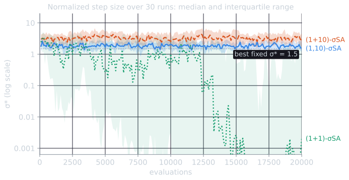
- The $(1+1)$-ES with a self-adapted step size has $\lambda/\mu = 1$, below $1/P_s \approx 3.7$. Its normalized step size $\sigma^* = \sigma n / R$ drifted down. At 15,000 evaluations it was below 0.005 in at least half the runs, against a best value of about 1.5, and the convergence rate was 28% of what the best fixed $\sigma^*$ achieves.
- The $(1+10)$-ES kept $\sigma^*$ at a median of 3.27, about twice the best value, while the $(1,10)$-ES, with the same $\lambda$ and $\tau$, kept it at 1.85 and converged 25% faster.
Measuring the pull on the step size
Both arguments can be made quantitative with a one-generation experiment. Place a parent at distance $R = 1$ from the optimum of the ten-dimensional sphere with a given $\sigma^*$, run one generation, and compare $\ln \sigma^*$ of the parent with $\ln \sigma^*$ of the individual that survives, $\sigma_{\text{new}}\, n / R_{\text{new}}$. The change has two sources: the survivor's step-size mutation $\tau\xi$, and the change of distance, since moving closer to the optimum raises $\sigma^*$ even if $\sigma$ stays the same. Averaging over 20,000 generations per point gives the expected drift of $\ln \sigma^*$:
| $\sigma^*$ | 0.5 | 1 | 1.5 | 2 | 3 | 4 | 6 | 8 |
|---|---|---|---|---|---|---|---|---|
| $(1,10)$ | +0.155 | +0.127 | +0.075 | +0.012 | −0.132 | −0.277 | −0.534 | −0.755 |
| $(1+10)$ | +0.153 | +0.134 | +0.086 | +0.037 | −0.033 | −0.054 | −0.034 | −0.013 |
| $(1+1)$ | +0.003 | +0.004 | +0.001 | −0.003 | −0.009 | −0.007 | −0.003 | −0.001 |
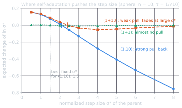
The table reads like a restoring force. For the $(1,10)$-ES the drift is positive below $\sigma^* \approx 2.1$ and negative above it, and it grows with the distance from that point: a parent with $\sigma^* = 8$ loses on average 0.755 in $\ln \sigma^*$, more than half its step size, in one generation. The selected offspring at $\sigma^* = 8$ had an average $\xi$ of −1.07, where the average over all offspring is 0, so selection picks step-size mutations from the lower tail. The equilibrium, 2.09 by interpolation, is a little above the best fixed value of 1.5, and the runs below held a median of 1.85.
The $(1+10)$-ES has the same pull for small step sizes, where most generations produce a better offspring and the plus and comma rules nearly coincide. For large step sizes the pull fades: the drift is −0.033 at $\sigma^* = 3$ and only −0.013 at 8, because most generations then produce no improvement, and the parent survives with its step size unchanged. Nothing pushes a too-large step size back down except the occasional lucky offspring, and the runs drifted to a median $\sigma^*$ of 3.27, above the zero crossing of the curve at 2.42: past that point the pull is too weak to bring a large step size back quickly. The $(1+1)$-ES has one offspring and no choice among step sizes at all: whether the single offspring is accepted depends on its position, and its $\xi$ is only weakly correlated with that. The drift never exceeds 0.01 in either direction, so $\ln \sigma^*$ performs a nearly free random walk, which in the runs ended with collapsed step sizes.
Derandomization and cumulative step-size adaptation
Self-adaptation selects step sizes only indirectly, through the positions they produce. Hansen and Ostermeier (2001, §§1–2) list the consequences. A better step size has only a higher probability of being selected, and the difference in probability can be small, so the selection of step sizes is very noisy. The mutation of the strategy parameters must be strong enough to make a difference in selection. Adapting $n$ individual step sizes, in their experience, requires a population that grows linearly with $n$. And they note that the global step size is often adapted to be too small, since the step size most likely to be selected is not the one that gives the most progress. (In the experiment below, most self-adaptive strategies erred in the other direction, with step sizes somewhat larger than the best.) Ostermeier, Gawelczyk, and Hansen (1994a) introduced a first level of derandomization: the strategy parameters are changed so as to make the selected mutation steps more likely again, directly, rather than through random mutation of the parameters and selection.
Cumulative step-size adaptation (CSA), also called cumulative path length control, goes a step further and uses the history of selected steps (Ostermeier, Gawelczyk, and Hansen, 1994b; Beyer and Schwefel, 2002, §4.3.3). Its reasoning is geometric (Hansen, 2016, §4). If consecutive selected steps point in similar directions, the same distance could be covered with fewer, longer steps, so $\sigma$ should grow. If they cancel each other out, $\sigma$ should shrink. If they are uncorrelated, as they would be under random selection, $\sigma$ is right. For a $(\mu/\mu, \lambda)$-ES with intermediate recombination and no covariance matrix, one generation is:
- Sample $\mathbf{z}_k \sim \mathcal{N}(\mathbf{0}, \mathbf{I})$ and $\mathbf{x}_k = \mathbf{m} + \sigma \mathbf{z}_k$ for $k = 1, \dots, \lambda$.
- Select the best $\mu$, set $\mathbf{m}$ to their mean, and let $\bar{\mathbf{z}}$ be the mean of their $\mathbf{z}_k$.
- Update the evolution path: $\mathbf{p} \leftarrow (1 - c)\, \mathbf{p} + \sqrt{c(2 - c)\mu} \; \bar{\mathbf{z}}$.
- Update the step size: $\sigma \leftarrow \sigma \exp\!\left( \frac{c}{d} \left( \frac{\lVert \mathbf{p} \rVert}{\mathrm{E}\lVert \mathcal{N}(\mathbf{0}, \mathbf{I}) \rVert} - 1 \right) \right)$.
The factor $\sqrt{c(2-c)\mu}$ makes $\mathbf{p}$ standard normal under random selection, so its length is compared with the expected length of a standard normal vector, approximately $\sqrt{n}\,(1 - 1/(4n) + 1/(21n^2))$. The constant $1/c$ is the time horizon of the path and $d \approx 1$ damps the change. Hansen (2016) gives the defaults $c = (\mu_{\text{eff}} + 2)/(n + \mu_{\text{eff}} + 5)$ and $d = 1 + 2\max(0, \sqrt{(\mu_{\text{eff}} - 1)/(n + 1)} - 1) + c$, where $\mu_{\text{eff}} = \mu$ for equal weights. Nothing in the update is random apart from the samples themselves, and no learning rate $\tau$ needs to be chosen. Beyer and Schwefel note the resemblance to the 1/5 rule: both use information gathered over several generations, but the 1/5 rule only counts successes, while CSA uses the directions of the steps. The same idea, applied to a covariance matrix, gives CMA-ES (Hansen and Ostermeier, 2001).
Experiment
Script: tools/experiments/evolution/self_adaptation.py. Dimension $n = 10$, the sphere $\sum x_i^2$ and the ellipsoid $\sum 10^{6(i-1)/(n-1)} x_i^2$ (condition number $10^6$), 30 runs per strategy (seeds 0 to 29), all parents starting at one point drawn from $[-2, 2]^{10}$ with $\sigma_0 = 1.2$, the same setup as the CMA-ES experiments. Single step sizes use $\tau = 1/\sqrt{n}$; the strategy with $n$ step sizes ("$n$SA") uses $\tau'$ and $\tau$ from eq. 27 with $c = 1$; recombination is intermediate for positions and step sizes; CSA uses Hansen's defaults with equal weights. The $(5/5, 10)$ strategies use the default population size of Hansen (2016) for $n = 10$, $\lambda = 4 + \lfloor 3 \ln n \rfloor = 10$. Budgets were 20,000 evaluations on the sphere and 100,000 on the ellipsoid.
To know what each strategy should aim for, the script first ran each population structure with $\sigma^*$ held fixed and measured the normalized convergence rate $n \cdot \Delta \ln R$ per evaluation (10 runs per value). The best values on its grid were $\sigma^* = 1.5$ for $(1+1)$ (rate 0.221), $(1,10)$ (0.137) and $(1+10)$ (0.137); 3 for $(5/5, 10)$ (0.123); and 6 for $(15/15, 100)$ (0.053) and $(15/15 + 100)$ (0.052). With $\sigma^*$ of 4 or more, the $(1,10)$-ES went backwards, while the $(1+10)$-ES only slowed down, which is the difference between comma and plus in its simplest form.
Sphere
Medians over 30 runs, interquartile ranges in parentheses. The rate is measured between 5,000 and 20,000 evaluations; $\sigma^*$ is the median over all generations of a run.
| Strategy | Evaluations to $f \le 10^{-8}$ | Normalized rate | Median $\sigma^*$ | Best fixed $\sigma^*$ (rate) |
|---|---|---|---|---|
| $(1+1)$-σSA | 1,171 (951–1,914) | 0.061 (0.030–0.076) | 0.65 (0.00–1.20) | 1.5 (0.221) |
| $(1,10)$-σSA | 1,116 (1,058–1,212) | 0.091 (0.090–0.092) | 1.85 (1.81–1.88) | 1.5 (0.137) |
| $(1+10)$-σSA | 1,371 (1,139–1,518) | 0.073 (0.069–0.077) | 3.27 (3.05–3.37) | 1.5 (0.137) |
| $(5/5,10)$-σSA | 1,232 (1,180–1,352) | 0.082 (0.081–0.083) | 2.18 (2.13–2.24) | 3 (0.123) |
| $(5/5,10)$-CSA | 2,172 (2,095–2,220) | 0.048 (0.047–0.049) | 4.79 (4.78–4.85) | 3 (0.123) |
| $(15/15,100)$-σSA | 3,351 (3,269–3,456) | 0.031 (0.030–0.031) | 8.16 (7.89–8.58) | 6 (0.053) |
| $(15/15+100)$-σSA | 3,628 (3,513–3,808) | 0.029 (0.029–0.030) | 9.67 (9.26–9.88) | 6 (0.052) |
| $(15/15,100)$-$n$SA | 6,658 (6,420–6,910) | 0.015 (0.015–0.015) | 11.09 (10.74–11.69) | 6 (0.053) |
| $(15/15,100)$-CSA | 11,147 (10,873–11,415) | 0.009 (0.009–0.010) | 14.96 (14.74–15.23) | 6 (0.053) |
The median $\sigma^*$ along the runs, at selected numbers of evaluations:
| Strategy | 500 | 1,000 | 2,000 | 5,000 | 10,000 | 20,000 |
|---|---|---|---|---|---|---|
| $(1+1)$-σSA | 2.16 | 2.01 | 0.93 | 0.27 | 1.02 | 0.00 |
| $(1,10)$-σSA | 1.75 | 1.99 | 1.76 | 1.67 | 2.05 | 1.50 |
| $(1+10)$-σSA | 3.09 | 2.37 | 3.09 | 3.52 | 2.56 | 2.82 |
| $(15/15,100)$-σSA | 6.44 | 7.43 | 8.74 | 8.98 | 8.29 | 8.52 |
| $(15/15,100)$-CSA | 16.16 | 14.16 | 15.59 | 16.33 | 14.58 | 15.38 |
All strategies converged linearly, and all except $(1+1)$-σSA held $\sigma^*$ at a steady level within the first 1,000 to 2,000 evaluations. Read against the calibration, these are our observations on this setup:
- Comma against plus. With one parent, comma selection gave a rate 25% higher than plus (0.091 against 0.073) and a $\sigma^*$ near the best value, while plus let it sit at about twice the best. With 15 parents and recombination the effect was smaller: 0.031 against 0.029, with $\sigma^*$ of 8.2 and 9.7.
- The $(1+1)$-ES does not self-adapt. Its step size wandered and then collapsed, and its rate varied by a factor of 2.5 across the middle half of the runs.
- Population size costs evaluations on the sphere. The best rate per evaluation falls from 0.137 for $\lambda = 10$ to 0.053 for $\lambda = 100$, because in ten dimensions a hundred offspring per generation are far more than the sphere needs. Populations pay off on multimodal and noisy functions, which this experiment does not test.
- CSA kept the step size larger than optimal here. With $(5/5, 10)$, CSA held $\sigma^*$ at 4.8 against a best value of 3 and converged at 0.048, against 0.082 for σSA; with $(15/15, 100)$ it held 15 against 6. Self-adaptation with $\tau = 1/\sqrt{n}$ was faster on the sphere in both configurations. The direction of the error is what theory predicts. Arnold and Beyer (2004) showed that on the sphere, in the limit of large $n$, the step size at which CSA's update is neutral is the optimal one, but since the distance to the optimum keeps shrinking and $\sigma$ adapts gradually, the step size actually realized stays behind that target and is too large, at a cost of about 17% of the optimal progress rate. In ten dimensions the loss was much larger. This is one function in one small dimension, and it does not contradict Hansen and Ostermeier's argument, which concerns reliability with small populations and the adaptation of many parameters at once; the ellipsoid shows where that matters.
- Learning $n$ step sizes has a price on the sphere, where they are not needed: the rate halved compared with one step size, 0.015 against 0.031.
Ellipsoid
On the ellipsoid with condition number $10^6$, no strategy with a single step size, whether self-adapted or controlled by CSA, came near the target. After 100,000 evaluations the median $\log_{10} f$ was between 1.6 and 2.5 for all eight of them: 2.5 for $(1+1)$-σSA, 1.8 for $(1,10)$-σSA, 1.6 for $(1+10)$-σSA, 2.2 for $(15/15,100)$-σSA, 1.9 for $(15/15+100)$-σSA, 2.3 for $(5/5,10)$-σSA, and 2.1 for both CSA strategies. Their step sizes fell steadily, to a geometric mean of $10^{-4.4}$ for $(1,10)$-σSA and $10^{-10.2}$ for $(1+1)$-σSA, limited by the steepest axis, as in the 1/5 rule experiment.
With $n$ step sizes the picture changed completely. All 30 runs of $(15/15,100)$-$n$SA reached $f \le 10^{-8}$, after a median of 11,630 evaluations (11,212–12,479), and the median $\log_{10} f$ at 100,000 evaluations was $-125.8$. The ratio $\sigma_1/\sigma_{10}$ between the step sizes on the flattest and the steepest axes ended at a median of 1,122 (847–1,390), close to $\sqrt{10^6} = 1{,}000$, the ratio that turns this ellipsoid into a sphere. The median $\log_{10}$ of the geometric mean step size was $-0.4$, $-1.8$, $-4.6$, $-11.4$, $-31.4$, and $-64.5$ at 2,000, 5,000, 10,000, 20,000, 50,000 and 100,000 evaluations. Once the shape had been learned, between 20,000 and 100,000 evaluations, $f$ fell by 1.33 decades per 1,000 evaluations, almost exactly the 1.30 that the same strategy achieved on the sphere between 5,000 and 20,000. The learning took the first 5,000 to 10,000 evaluations.
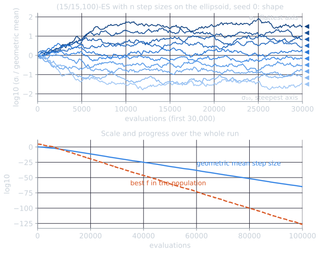
In this run the ratio $\sigma_1/\sigma_{10}$ first exceeded 100 after 4,200 evaluations and 1,000 after 8,000. The ideal spacing follows from the ellipsoid's coefficients $10^{6(i-1)/9}$: the step size along axis $i$ should be proportional to $1/\sqrt{10^{6(i-1)/9}} = 10^{-(i-1)/3}$, a third of a decade between neighbors. The fan in the top panel is not perfectly even. The step sizes keep mutating, and only their effect on $f$ is selected, so neighboring step sizes swap places from time to time; what selection maintains is the overall spread.
This works only because the ellipsoid is aligned with the coordinate axes. Rotate it, and individual step sizes no longer help; that is the case for which correlated mutations were proposed and for which CMA-ES is designed.
Plus and comma under noise
A common heuristic argument for comma selection on noisy problems runs as follows: a plus strategy can be trapped by a parent whose quality was overestimated by a lucky evaluation, since that parent is compared against every new offspring and never re-evaluated. A small experiment of our own shows that, at least in one setup, the trade-off is less one-sided than the argument suggests. The sphere in ten dimensions is observed with log-normal noise, $f(\mathbf{x})\, e^{\varepsilon N(0,1)}$, a fresh draw for every evaluation, so that the noise is a constant fraction of $f$ however close the search comes. The $(1,10)$-σSA and $(1+10)$-σSA strategies of the experiment above ran for 20,000 evaluations, 30 runs each, with a plus parent keeping the noisy value it was selected with. Median $\log_{10}$ of the true $f$ of the parent, interquartile range in brackets:
| Noise $\varepsilon$ | Strategy | 2,000 evaluations | 20,000 evaluations | Last parent replaced at generation | Stored / true value at end |
|---|---|---|---|---|---|
| 0.25 | $(1,10)$ | −3.4 [−5.2, −2.0] | −16.9 [−30.3, −6.6] | 2,000 | 0.67 |
| 0.25 | $(1+10)$ | −3.8 [−5.4, −1.8] | −29.8 [−41.2, −15.7] | 1,818 | 0.42 |
| 0.5 | $(1,10)$ | 1.2 [0.9, 1.5] | 0.1 [−1.1, 1.3] | 2,000 | 0.45 |
| 0.5 | $(1+10)$ | 0.1 [−0.4, 0.5] | −3.2 [−5.6, −1.1] | 1,762 | 0.19 |
| 1.0 | $(1,10)$ | 3.1 [2.3, 4.0] | 4.7 [3.4, 7.3] | 2,000 | 0.20 |
| 1.0 | $(1+10)$ | 1.3 [1.1, 1.5] | 1.3 [0.8, 1.5] | 832 | 0.02 |
(Starting points drawn from $[-2, 2]^{10}$ have $f = 13.3$ on average, $\log_{10} f \approx 1.1$. The generation of the last replacement is a median over runs; a comma parent is replaced in every generation, so for comma selection it is always the last one, 2,000.)
Both effects of noise are visible, and they pull in opposite directions. The plus strategy's parent is overvalued, increasingly so as the noise grows: at $\varepsilon = 1$ its stored value is a median of 50 times better than its true value, no offspring can beat it, and its last replacement came at generation 832 of 2,000. It stagnates. The comma strategy cannot stagnate in that way, but it fails differently. Every generation must accept the apparent best even when it is truly worse, and, in our reading, selection among offspring becomes partly selection on noise, so it no longer prefers good step sizes reliably. With $\varepsilon = 0.5$ it gained only about one order of magnitude in 20,000 evaluations, and with $\varepsilon = 1$ it drifted away from the optimum, ending farther from it than it started. At low and moderate noise in this setup the plus strategy was better, and at $\varepsilon = 1$ neither made progress. One experiment with one noise model and no re-evaluation does not settle the general question, but it shows that neither selection scheme handled strong noise by itself here. The remedies usually suggested, such as re-evaluating the parent, averaging several evaluations, or enlarging the population with recombination so that averaging cancels part of the noise, were not tested here.
Summary
Self-adaptation turns the step size into part of the genome and lets selection set it. It needs a birth surplus and works best with comma selection, which penalizes step sizes that are too large instead of preserving them. With a single step size it tracks the scale of the problem; with $n$ step sizes it can learn an axis-parallel scaling, at the cost of slower adaptation and larger populations; with rotation angles it can in principle learn any normal distribution, but the angles and step sizes disturb each other. Cumulative step-size adaptation replaces the random mutation of $\sigma$ by a deterministic update from the evolution path. In this experiment that did not make it faster on the sphere, but it is the ingredient that, together with covariance matrix adaptation, solves the problems self-adaptation struggles with. Natural evolution strategies reach a similar algorithm from a different starting point, the gradient of expected fitness with respect to the parameters of the search distribution.
References
- Arnold, D. V., and Beyer, H.-G. (2004). Performance analysis of evolutionary optimization with cumulative step length adaptation. IEEE Transactions on Automatic Control, 49(4), 617–622.
- Beyer, H.-G. (1995). Toward a theory of evolution strategies: On the benefits of sex, the $(\mu/\mu, \lambda)$ theory. Evolutionary Computation, 3(1), 81–111.
- Beyer, H.-G., and Schwefel, H.-P. (2002). Evolution strategies: A comprehensive introduction. Natural Computing, 1(1), 3–52.
- Eiben, A. E., and Smith, J. E. (2015). Introduction to Evolutionary Computing, 2nd ed. Springer.
- Hansen, N. (2016). The CMA evolution strategy: A tutorial. arXiv:1604.00772.
- Hansen, N., and Ostermeier, A. (2001). Completely derandomized self-adaptation in evolution strategies. Evolutionary Computation, 9(2), 159–195.
- Ostermeier, A., Gawelczyk, A., and Hansen, N. (1994a). A derandomized approach to self-adaptation of evolution strategies. Evolutionary Computation, 2(4), 369–380.
- Ostermeier, A., Gawelczyk, A., and Hansen, N. (1994b). Step-size adaptation based on non-local use of selection information. In Y. Davidor, H.-P. Schwefel and R. Männer (eds.), Parallel Problem Solving from Nature: PPSN III, Lecture Notes in Computer Science 866, 189–198. Springer.
- Rechenberg, I. (1994). Evolutionsstrategie '94. Frommann-Holzboog.
- Rudolph, G. (1992). On correlated mutations in evolution strategies. In R. Männer and B. Manderick (eds.), Parallel Problem Solving from Nature 2, 105–114. Elsevier.
- Schwefel, H.-P. (1975). Evolutionsstrategie und numerische Optimierung. Doctoral dissertation, Technical University of Berlin.
- Schwefel, H.-P. (1977). Numerische Optimierung von Computer-Modellen mittels der Evolutionsstrategie. Birkhäuser.
- Schwefel, H.-P. (1981). Numerical Optimization of Computer Models. Wiley.
- Schwefel, H.-P. (1995). Evolution and Optimum Seeking. Wiley.