Four documents have probabilities of relevance 0.2, 0.9, 0.5, and 0.6, and a user will read some number of them from the top of a list. In what order should they be shown? Intuition says highest probability first, and the intuition is right. The Probability Ranking Principle (PRP) states it precisely, and under stated conditions no other ordering does better. The principle is the theoretical justification for ranked retrieval. Every model in this topic, from the Binary Independence Model to BM25, is an attempt to estimate the quantity the PRP says to sort by.
The idea that retrieval should rank by probability of relevance goes back to Maron and Kuhns (1960). Stephen Robertson (1977) gave the principle its standard statement, which he credited to William Cooper, and showed that it is optimal under certain assumptions but can fail when they do not hold. This article states the principle, proves why it holds, extends it to unequal costs, works through an example where it fails, and examines the assumptions it depends on, following Manning, Raghavan, and Schütze (2008, §11.2). The probability primer reviews the notation. The numbers in the examples are computed by tools/experiments/cranfield/prp_examples.py.
The principle
Treat the relevance of document $d$ to query $q$ as a binary random variable $R$, equal to 1 if $d$ is relevant and 0 otherwise. The system cannot observe $R$. It observes only representations of the document and the query, from which it can at best estimate $P(R = 1 \mid d, q)$. Robertson's statement of the principle:
If a reference retrieval system's response to each request is a ranking of the documents in the collection in order of decreasing probability of relevance to the user who submitted the request, where the probabilities are estimated as accurately as possible on the basis of whatever data have been made available to the system for this purpose, the overall effectiveness of the system to its user will be the best that is obtainable on the basis of those data.
Why the ordering is optimal
Suppose the user reads the top $k$ documents, for some $k$ the system does not know in advance. The expected number of relevant documents among them is the sum of their probabilities of relevance, so the expected precision at $k$ is the average of those probabilities. For the four documents above:
| Ordering | P@1 | P@2 | P@3 | P@4 |
|---|---|---|---|---|
| By probability: 0.9, 0.6, 0.5, 0.2 | 0.900 | 0.750 | 0.667 | 0.550 |
| As given: 0.2, 0.9, 0.5, 0.6 | 0.200 | 0.550 | 0.533 | 0.550 |
For any fixed $k$, the sum of $k$ probabilities is largest when it includes the $k$ largest, which is what sorting puts at the top. Sorting achieves this for every $k$ at once, so the sorted list maximizes expected precision at every cutoff simultaneously, wherever the user stops. At $k = 4$ the two orderings tie, because both include all four documents. The order matters only for users who stop earlier, which is nearly all of them.
The argument step by step
The claim "best at every cutoff at once" is stronger than it first sounds, so it is worth proving rather than asserting. Two facts carry the proof.
- Expectation is additive. Let $R_i$ be the relevance of the document at position $i$. The number of relevant documents in the top $k$ is $R_1 + \dots + R_k$, and its expectation is $p_1 + \dots + p_k$, whatever the dependence between the $R_i$. Expected precision at $k$ is this sum divided by $k$.
- An adjacent swap changes one cutoff. Take any ordering in which a document with probability $p_i$ sits directly above one with a larger probability $p_{i+1}$. Swap the two. For every cutoff $k < i$ neither document is in the top $k$, and for every $k > i$ both are, so those sums are unchanged. Only the cutoff $k = i$ changes: its top set now contains $p_{i+1}$ instead of $p_i$, and its sum rises by $p_{i+1} - p_i > 0$.
- Sort by repeated swaps. Any ordering can be turned into the sorted one by repeatedly swapping adjacent pairs that are out of order, as bubble sort does. Each swap raises one cutoff's expected precision and leaves the others unchanged.
- Conclusion. The sorted ordering is at least as good as every other ordering at every cutoff, so it is optimal for a user who stops at any $k$, and for any mixture of users who stop at different depths.
For the example, the ordering 0.9, 0.5, 0.6, 0.2 has one pair out of order. Its expected relevant counts at $k = 1, \dots, 4$ are 0.9, 1.4, 2.0, 2.2, against 0.9, 1.5, 2.0, 2.2 for the sorted order: the single swap that fixes it changes only $k = 2$, by $0.6 - 0.5$. Step 1 is where the argument's assumptions hide. Additivity holds for any dependence, but it makes the expected number of relevant documents the measure of success. A user who wants one good answer is not served by an expectation, as the ambiguous query below shows.
The same idea as a decision
The same reasoning applied to a single decision gives the Bayes optimal decision rule under 1/0 loss, where each retrieved nonrelevant document and each missed relevant document costs one unit. Retrieve $d$ if and only if
$$P(R = 1 \mid d, q) > P(R = 0 \mid d, q),$$
that is, if the document is more likely relevant than not. This is the decision a classifier makes. The PRP is the ranking version of the same idea, and Manning, Raghavan, and Schütze (2008, Theorem 11.1) state the result as minimizing expected loss under 1/0 loss.
The two views meet when a system must return a set rather than a list. If it returns the top $k$ of the sorted four, the expected loss is the expected number of nonrelevant documents returned plus the expected number of relevant documents left out:
| Documents returned | none | top 1 | top 2 | top 3 | all 4 |
|---|---|---|---|---|---|
| Expected loss | 2.2 | 1.4 | 1.2 | 1.2 | 1.8 |
The loss falls while the next document is more likely relevant than not (0.9, then 0.6) and rises once it is less likely (0.2). The document with probability exactly 0.5 costs as much to include as to leave out, which is why the top-2 and top-3 sets tie. Returning the top of the sorted list and stopping where the probability crosses one half is the Bayes rule.
The principle with retrieval costs
Errors are rarely equally expensive. In legal discovery or a systematic medical review, missing a relevant document is far worse than reading an extra nonrelevant one. In a casual web search the reverse is closer to true. Let $C_1$ be the cost of failing to retrieve a relevant document and $C_0$ the cost of retrieving a nonrelevant one. Writing $p_d = P(R = 1 \mid d, q)$, the generalized PRP says that document $d$ should be retrieved next if, for every document $d'$ not yet retrieved,
$$C_0 (1 - p_d) - C_1\, p_d \;\le\; C_0 (1 - p_{d'}) - C_1\, p_{d'}.$$
The left side is the net expected cost of retrieving $d$: the cost of retrieving it if it is nonrelevant, minus the cost saved by not missing it if it is relevant. The expression decreases as $p_d$ increases, so for positive costs the generalized rule produces the same ordering as the basic one.
What the costs change is where to stop. Retrieving a document is worthwhile when its net expected cost is negative:
$$C_0 (1 - p_d) < C_1\, p_d \quad\Longleftrightarrow\quad p_d > \frac{C_0}{C_0 + C_1}.$$
With equal costs the threshold is 0.5, the Bayes rule above. If missing a relevant document is nine times as costly as reading a nonrelevant one, $C_1 = 9 C_0$, the threshold falls to $1/10$: every document with more than a 10 percent chance of relevance is worth reviewing. This is the decision a filtering system or a technology-assisted legal review must make (see search in professional domains). It depends on the costs, not on the ranking.
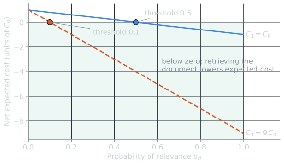
The threshold is the one place where the PRP needs calibrated probabilities. To decide whether a document's probability exceeds 0.1, the score must actually be a probability. A ranking function such as BM25, whose scores are not probabilities, can produce the right order and still give no guidance on where to stop.
Where the principle fails: an ambiguous query
The proof above maximizes the expected number of relevant documents. Users often want something else: one document that answers the question. When the relevance of documents is correlated, those two goals pull apart, and the PRP can be the wrong ordering.
Consider a query with two senses, such as jaguar the car and jaguar the animal. Suppose 60 percent of the users who type it mean the car and 40 percent the animal. Four documents are candidates: three about the car (A1, A2, A3), each relevant exactly when the user means the car, and one about the animal (B), relevant exactly when the user means the animal. Each A document has probability of relevance 0.6, and B has 0.4. The PRP ranks A1, A2, A3, B. A diversified ranking puts B second.
| Ordering | E[relevant in top 2] | P(at least one relevant in top 2) |
|---|---|---|
| PRP: A1, A2, A3, B | 1.2 | 0.6 |
| Diverse: A1, B, A2, A3 | 1.0 | 1.0 |
The PRP order wins on the measure it was proved for. Car users find two relevant documents in the top two, so the expectation is $2 \times 0.6 = 1.2$. But the 40 percent of users who meant the animal find nothing until position four. The diverse order gives every user at least one relevant document in the top two. Over all 24 orderings, 1.2 is the most relevant documents expected in the top two and 1.0 the highest probability of at least one; the PRP order achieves the first and not the second.
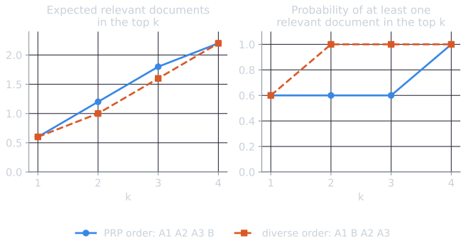
The failure comes from step 1 of the proof. The relevance of A1, A2, and A3 is not independent: if A1 is irrelevant to a user, so are A2 and A3. The PRP scores each document as if it were alone, so it cannot see that the second car document adds nothing for the users the first one failed. This is an instance of the failure Robertson (1977) already allowed for, optimality only while the assumptions hold, and the kind of case that motivates the diversity methods discussed below.
Assumptions the proof depends on
The optimality result holds only under assumptions that real search rarely satisfies. Knowing which ones fail explains much of the later history of the field.
- The probabilities are known. The proof assumes the system has $P(R = 1 \mid d, q)$, not an estimate of it. In practice the probabilities come from a model, and a ranking is only as good as its estimates. Robertson's statement already hedges on this point, promising only the best effectiveness obtainable from the data available.
- Relevance is independent across documents. The PRP scores each document in isolation. If the top three results are near-duplicates, the second and third add almost nothing for the user, but the PRP ranks them highly anyway. The ambiguous query above is the same problem in its sharpest form. This motivates diversity-aware ranking such as maximal marginal relevance (Carbonell and Goldstein, 1998), which penalizes a candidate for similarity to documents ranked above it, as described in how a web search engine answers a query.
- Relevance is binary. Users experience degrees of usefulness. Measures such as nDCG were designed for graded relevance, and learning-to-rank methods optimize them directly rather than a binary probability.
- The user reads top-down at uniform cost. Interfaces with snippets, images, and answer boxes break the linear reading model the proof relies on.
None of this makes the PRP wrong. It makes it a statement about an idealized setting, and the useful question for any ranking model becomes how closely its scores track the true probability of relevance.
Estimating the probability
The PRP gives no recipe for computing $P(R = 1 \mid d, q)$. With unlimited relevance judgments one could estimate it directly for each query-document pair, but judgments are expensive and the space of queries is effectively unbounded. Models therefore estimate it from features of the document and query, most simply from which query terms the document contains.
- The Binary Independence Model represents each document by the presence or absence of terms, assumes conditional independence, and derives a ranking that is monotonic in the probability of relevance.
- Okapi BM25 keeps the probabilistic framing while adding term frequency and document length.
- Inference networks compute a belief that the information need is met by propagating probabilities through a network of documents, concepts, and query operators.
- Language models rank by a different quantity, $P(q \mid d)$, which can be connected back to the PRP under further assumptions.
A convenient consequence of the principle is that a model never needs calibrated probabilities to rank correctly. Any score that is a monotonic function of $P(R = 1 \mid d, q)$ produces the same ordering. The derivation of the BIM uses this freedom at every step. It replaces probabilities with odds, drops factors that are constant for a query, and takes logarithms. Calibration matters only when the scores themselves are used, as in the stopping threshold above.
References
- Carbonell, J., and Goldstein, J. (1998). The use of MMR, diversity-based reranking for reordering documents and producing summaries. In Proceedings of SIGIR 1998, 335–336.
- Manning, C. D., Raghavan, P., and Schütze, H. (2008). Introduction to Information Retrieval, section 11.2. Cambridge University Press.
- Maron, M. E., and Kuhns, J. L. (1960). On relevance, probabilistic indexing and information retrieval. Journal of the ACM, 7(3), 216–244.
- Robertson, S. E. (1977). The probability ranking principle in IR. Journal of Documentation, 33(4), 294–304.