Basic TF-IDF multiplies a term's raw count in a document by its inverse document frequency. Two of its assumptions do not hold up. The first is that importance grows in proportion to count, so a term occurring twenty times is twenty times as significant as one occurring once. The second, once cosine normalization is applied, is that dividing by a document's vector length makes documents of every length equally likely to be retrieved. Experiments on test collections from the 1970s onward produced a family of variants that correct both. This article describes the main ones, following Manning, Raghavan, and Schütze (2008, §6.4), and the compact notation the SMART system used to name combinations of them.
Sublinear term frequency
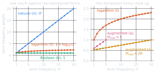
A document that uses a term twenty times is probably more about it than one that uses it once, but not twenty times more. Sublinear term frequency dampens the count with a logarithm:
$$\mathit{wf}_{t,d} = \begin{cases} 1 + \log_{10} \mathit{tf}_{t,d} & \text{if } \mathit{tf}_{t,d} > 0, \\ 0 & \text{otherwise.} \end{cases}$$
| $\mathit{tf}$ | 1 | 2 | 10 | 20 | 100 |
|---|---|---|---|---|---|
| $\mathit{wf}$ | 1.0 | 1.3 | 2.0 | 2.3 | 3.0 |
Each tenfold increase in count adds only 1 to the weight. The TF-IDF weight becomes $\mathit{wf}_{t,d} \times \mathit{idf}_t$. The "1 +" matters: without it a term occurring once would get $\log 1 = 0$, the same as a term that does not occur.
The effect on ranking can be large. For the query car insurance, with the Reuters IDF values from TF-IDF weighting (car 1.65, insurance 1.62), compare three documents:
| Document | Raw TF-IDF score | Sublinear score |
|---|---|---|
| A: car 100 times, no insurance | 165.00 | 4.95 |
| B: car once, insurance once | 3.27 | 3.27 |
| C: car 10 times, insurance twice | 19.74 | 5.41 |
With raw counts, document A, which never mentions insurance, outscores C by more than eight times. With sublinear weights, C, which matches both query terms, ranks first. Repetition still counts, but it can no longer outweigh matching more of the query. The novels example showed the same effect on document-to-document similarity.
Maximum term frequency normalization
Another approach normalizes each term frequency by the largest term frequency in the same document:
$$\mathit{ntf}_{t,d} = a + (1 - a)\,\frac{\mathit{tf}_{t,d}}{\mathit{tf}_{\max}(d)},$$
where $\mathit{tf}_{\max}(d)$ is the frequency of the document's most frequent term and $a$ is a smoothing constant, typically 0.4 or 0.5. The smoothing keeps any term that occurs from getting a weight near zero. With $a = 0.4$ and $\mathit{tf}_{\max} = 10$, a term occurring once gets 0.46, five times 0.7, and ten times 1.0.
The idea is that a long document repeats everything more often, so its counts should be scaled relative to its own most frequent term. The method has known weaknesses (Manning, Raghavan, and Schütze, 2008, §6.4.2). A single unusually frequent term, such as a name repeated throughout a document, lowers the weights of all the others. And it cannot tell apart documents whose term frequencies are distributed very differently: a document with one dominant term and one whose terms are spread evenly can receive similar weights, although they probably differ in what they are about. It is used less than the other variants. Augmented term frequency, its form with $a = 0.5$, appears in classic query weighting schemes.
In the running example of this topic (introduced in TF-IDF weighting), the car review $d_2$ has counts car 5, best 2 and auto 1, so $\mathit{tf}_{\max} = 5$ and the augmented weights are $0.5 + 0.5 \times 5/5 = 1.0$, $0.5 + 0.5 \times 2/5 = 0.7$ and $0.5 + 0.5 \times 1/5 = 0.6$. Five occurrences of car now count less than twice one occurrence of auto.
The SMART notation
The SMART system named each weighting scheme with three letters for documents and three for queries, written ddd.qqq. The first letter gives the term frequency component, the second the document frequency component, and the third the normalization (Manning, Raghavan, and Schütze, 2008, §6.4.3). Salton and Buckley (1988) used an earlier version of the notation with different letters, in which their recommended scheme is written tfc.nfx. The letters below follow the later SMART usage:
| Letter | Term frequency | Letter | Document frequency | Letter | Normalization |
|---|---|---|---|---|---|
| n | natural: $\mathit{tf}$ | n | none: 1 | n | none |
| l | logarithm: $1 + \log \mathit{tf}$ | t | IDF: $\log(N/\mathit{df})$ | c | cosine |
| a | augmented: $0.5 + 0.5\,\mathit{tf}/\mathit{tf}_{\max}$ | p | probabilistic IDF: $\max(0, \log\frac{N - \mathit{df}}{\mathit{df}})$ | u | pivoted unique |
| b | Boolean: 1 if $\mathit{tf} > 0$ | b | byte size |
A weight is the product of the first two components, divided by the third. Reading a name is mechanical: ltc means "logarithmic term frequency, times IDF, then cosine normalization", and nnn means the raw count. The score of a document is the dot product of its weight vector with the query's.
A widely used combination is lnc.ltc. Documents get logarithmic term frequency, no IDF, and cosine normalization. Queries get logarithmic term frequency, IDF, and cosine normalization. Putting IDF only on the query side is enough, since every query term's weight multiplies the corresponding document weight. It also means document weights do not change when the collection, and therefore every document frequency, changes.
A worked lnc.ltc example
Manning, Raghavan, and Schütze (2008, Example 6.4 in §6.3.2) score the query best car insurance against a document containing auto and car once and insurance twice, such as car insurance auto insurance, using hypothetical document frequencies in a collection of $N = 1{,}000{,}000$ documents. They use a simpler weighting; under lnc.ltc the calculation is:
| Term | $\mathit{df}$ | Query: $\mathit{tf}$ | Query: $\mathit{tf}$ weight × IDF | Query: normalized | Document: $\mathit{tf}$ | Document: $1 + \log \mathit{tf}$ | Document: normalized | Product |
|---|---|---|---|---|---|---|---|---|
| auto | 5,000 | 0 | 0 | 0 | 1 | 1.0 | 0.52 | 0 |
| best | 50,000 | 1 | 1 × 1.3 = 1.3 | 0.34 | 0 | 0 | 0 | 0 |
| car | 10,000 | 1 | 1 × 2.0 = 2.0 | 0.52 | 1 | 1.0 | 0.52 | 0.27 |
| insurance | 1,000 | 1 | 1 × 3.0 = 3.0 | 0.78 | 2 | 1.3 | 0.68 | 0.53 |
The query vector's length is $\sqrt{1.3^2 + 2.0^2 + 3.0^2} \approx 3.83$, and the document's is $\sqrt{1^2 + 1^2 + 1.3^2} \approx 1.92$. The score is the sum of the products, $0.27 + 0.53 = 0.80$. Insurance contributes most: it has the highest IDF, so it carries the most weight in the query, and it occurs twice in the document.
The same scheme on the running example
The running example's query is the same, best car insurance, with IDFs from its own four documents: 0.125 for best and car, 0.301 for insurance. Each query term occurs once, so its ltc weight is its IDF divided by the query length, $\sqrt{0.125^2 + 0.125^2 + 0.301^2} \approx 0.349$, which gives 0.358, 0.358 and 0.862. On the document side, take the auto-insurance page $d_3$ (auto 3, best 1, insurance 2):
| Term | $d_3$: $\mathit{tf}$ | $1 + \log \mathit{tf}$ | normalized (÷ 2.208) | query ltc | product |
|---|---|---|---|---|---|
| auto | 3 | 1.477 | 0.669 | 0 | 0 |
| best | 1 | 1.000 | 0.453 | 0.358 | 0.162 |
| car | 0 | 0 | 0 | 0.358 | 0 |
| insurance | 2 | 1.301 | 0.589 | 0.862 | 0.508 |
The document length is $\sqrt{1.477^2 + 1^2 + 1.301^2} \approx 2.208$, and the score is $0.162 + 0.508 = 0.670$. The headline $d_1$ has three terms that each occur once, so each normalized weight is $1/\sqrt{3} \approx 0.577$, and its score is $0.577 \times (0.358 + 0.862) \approx 0.705$. (Values rounded to three decimals.)
Eight schemes on one collection
The table scores the running example under eight schemes, from the raw overlap count to fully dampened and normalized weights. The first row is the overlap score and the second the TF-IDF score of TF-IDF weighting; the documents a reader would want are $d_1$ and $d_3$.
| Scheme | $d_1$ | $d_2$ | $d_3$ | $d_4$ | Ranking |
|---|---|---|---|---|---|
| nnn.bnn | 2.000 | 7.000 | 3.000 | 5.000 | $d_2, d_4, d_3, d_1$ |
| ntn.bnn | 0.426 | 0.875 | 0.727 | 0.625 | $d_2, d_3, d_4, d_1$ |
| ntn.ntn | 0.106 | 0.109 | 0.197 | 0.078 | $d_3, d_2, d_1, d_4$ |
| ntc.ntc | 0.686 | 0.425 | 0.516 | 0.086 | $d_1, d_3, d_2, d_4$ |
| ltc.ltc | 0.686 | 0.333 | 0.632 | 0.114 | $d_1, d_3, d_2, d_4$ |
| lnc.ltc | 0.705 | 0.455 | 0.670 | 0.339 | $d_1, d_3, d_2, d_4$ |
| anc.atc | 0.705 | 0.447 | 0.655 | 0.331 | $d_1, d_3, d_2, d_4$ |
| bnc.btc | 0.705 | 0.413 | 0.705 | 0.358 | $d_1 = d_3, d_2, d_4$ |
Reading down the table, one component at a time:
- IDF (nnn to ntn) moves $d_3$ up, because its query match is on insurance, the rarer term. Putting IDF on the query side as well (ntn.ntn) squares its effect and moves $d_3$ to first.
- Cosine normalization (ntn to ntc) puts the short headline $d_1$ first. Without it, $d_1$ had the smallest weights because every count in it is 1.
- Logarithmic term frequency (ntc to ltc) leaves $d_1$ unchanged, since all its counts are 1, cuts the car review $d_2$ from 0.425 to 0.333, since its five occurrences of car now weigh $1 + \log 5 \approx 1.70$, and lifts $d_3$.
- Dropping IDF from documents (ltc to lnc) helps the car-loan page $d_4$ most, from 0.114 to 0.339. Under ltc, the rare term loan had a large weight, which made $d_4$'s vector long and every other component of it small after normalization. IDF on the document side affects scores even through terms the query does not contain, because they enter the length.
- Boolean term frequency (bnc.btc) discards counts entirely. $d_1$ and $d_3$ then tie at 0.705: each has three distinct terms and matches two of the query's three.
Once lengths are normalized, every scheme in the table agrees on the order $d_1$, $d_3$, $d_2$, $d_4$, and they differ only in the margins. On real collections the differences are larger, and they are measured with evaluation on test collections rather than read off one query. The demo in cosine similarity computes any of these schemes on the running example and on edited versions of it.
Pivoted length normalization
Cosine normalization makes a document's score independent of its length, which sounds fair. Singhal, Buckley, and Mitra (1996) tested whether it is. They grouped the documents of TREC collections by length and compared, for each group, the probability that a document in the group was relevant with the probability that it was retrieved under cosine normalization. Long documents turned out to be relevant more often than cosine normalization retrieved them, and short documents less often. Longer documents tend to cover more topics or cover one topic more fully, so they are more likely to contain what a searcher wants. Cosine normalization penalizes them too heavily.
Measuring the mismatch
The measurement itself is simple (Singhal, Buckley, and Mitra, 1996, §2.1). For TREC disks one and two, 741,856 documents, they sorted the documents by length in bytes and cut the list into bins of 1,000. For 50 queries they took the 9,805 pairs of a query and a relevant document and counted how many fell in each bin, which estimates $P(D \in \text{bin} \mid D \text{ relevant})$. They then retrieved the top 1,000 documents for each query with lnc.ltc and counted in the same way, which estimates $P(D \in \text{bin} \mid D \text{ retrieved})$. Plotted against the bins' median lengths, the two curves cross. Below the crossing point, short documents were retrieved more often than they were relevant; above it, long documents less often.
The correction, derived
The higher a document's normalization factor, the lower its scores, and so the lower its chance of being retrieved. To retrieve long documents more often, their factor must go down; to retrieve short documents less often, theirs must go up; and at the crossing point it should stay as it is. The simplest function that does this is a straight line through the old factor at the crossing point, tilted to be flatter than the identity. Call the crossing point the pivot $p$ and the new line's gradient the slope $s$. The line through $(p, p)$ with gradient $s$ is
$$\text{pivoted factor} = p + s\,(\text{old factor} - p) = (1 - s)\,p + s \times \text{old factor},$$
which is Equation 1 of Singhal, Buckley, and Mitra (1996, §2.2). Where cosine normalization divides by the vector length $\lvert \vec{V}(d) \rvert$, pivoted normalization divides by
$$(1 - s)\,p + s\,\lvert \vec{V}(d) \rvert,$$
where $p$ is typically the average vector length in the collection and $s < 1$. With $s = 1$ this is ordinary cosine normalization. With $s < 1$, a document of exactly average length is unaffected, shorter documents are divided by more than their length, and longer documents by less. With $p = 10$ and $s = 0.75$:
| Vector length | Cosine divisor | Pivoted divisor | Effect on score |
|---|---|---|---|
| 5 | 5 | 6.25 | × 0.80 |
| 10 | 10 | 10.0 | unchanged |
| 20 | 20 | 17.5 | × 1.14 |
| 40 | 40 | 32.5 | × 1.23 |
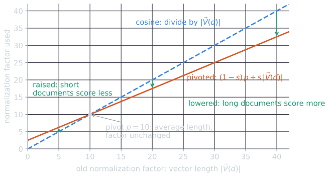
Two parameters remain, and one of them can be removed (Singhal, Buckley, and Mitra, 1996, §2.3). Multiplying every document's weights by the same constant does not change the ranking. Multiply them by $p$ and divide the denominator by $p$ as well:
$$\frac{w}{(1 - s)\,p + s\,\lvert \vec{V}(d) \rvert} \;\propto\; \frac{w}{(1 - s) + s\,\dfrac{\lvert \vec{V}(d) \rvert}{p}}.$$
With $p$ set to the average length, the denominator is $(1 - s) + s \times (\text{length} / \text{average length})$. A document of average length is divided by exactly 1, and only the slope has to be learned. This is the same form as the length component of BM25, $(1 - b) + b \times \mathit{dl} / \mathit{avdl}$, where the parameter $b$ plays the role of the slope.
What the original experiments found
The slope is tuned on a collection with relevance judgments, so that the probability of retrieval tracks the probability of relevance across lengths. With the pivot set to the average cosine factor of TREC disks one and two (13.36), the best slope for TREC queries 151 to 200 was 0.75, which raised average precision by 11.7% over cosine normalization; on queries 1 to 150 the best slope was 0.70, for an improvement of 11.9% (Singhal, Buckley, and Mitra, 1996, Tables 1 and 2). A slope learned on one query set worked nearly as well on the other.
Analysing the cosine factor itself, they observed that with $1 + \log \mathit{tf}$ weights most terms have weights close to 1, so the cosine factor of a document behaves roughly like the square root of its number of distinct terms, and on TREC it varied like that number raised to the power 0.6 (§4). They argued that the chance of a match grows linearly with the number of distinct terms, so a normalization should too. Pivoted unique normalization therefore pivots the number of distinct terms instead of the vector length, and pairs it with a term frequency weight divided by the document's average term frequency, $\frac{1 + \log \mathit{tf}}{1 + \log(\text{average } \mathit{tf})}$, so that a term occurring an average number of times counts 1 (§5). This is the "u" normalization of the SMART notation. They called the new term frequency factor L, and the document weighting Lnu. On queries 151 to 200 it improved average precision by 18.3% over cosine normalization and by 6.0% over the best pivoted cosine (Table 3).
Repeating the analysis on Cranfield
The analysis is easy to repeat on a small collection. Cranfield has 1,400 short abstracts of aeronautics papers and 225 queries with graded relevance judgments. Sorting the documents by their number of distinct terms (after stop-word removal and Porter stemming) and cutting them into 14 bins of 100, then comparing the bins of the 1,612 relevant (query, document) pairs with the bins of the top 10 documents retrieved by lnc.ltc for every query, gives the left panel below.
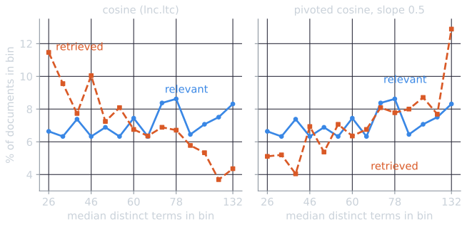
The pattern Singhal and colleagues found on TREC appears here too: cosine normalization favours the shortest abstracts and neglects the longest. Pivoting fixes the pattern but buys less effectiveness. Choosing the slope on the odd-numbered queries (the best was 0.50, with the pivot at the mean lnc vector length, 9.31) and testing on the even-numbered ones raised mean average precision from 0.294 to 0.297, about 1%. Over all 225 queries, the best slope, 0.60, gave 0.306 against 0.294, about 4%, but that figure tunes and tests on the same queries. Pivoted unique normalization, tuned the same way (slope 0.30), scored 0.292 on the even-numbered queries, slightly below cosine. Cranfield's abstracts span a narrow range of lengths, from 26 to 131.5 distinct terms at the bin medians, so there is less length bias to correct than in TREC, where the bin medians run from a few hundred bytes to more than 100 kilobytes (Singhal, Buckley, and Mitra, 1996, Figure 1). How much a length correction helps depends on how varied the collection's lengths are, which is the point Salton and Buckley made about weighting schemes in general.
Choosing a scheme
Salton and Buckley (1988) compared many combinations of these components on several test collections. Their general recommendations were to use term frequency with IDF and cosine normalization for documents, and augmented term frequency with IDF for queries, while noting that the best choice depends on the collection, especially on how long and varied its documents are. Later work replaced fixed choices with tuned parameters, as in pivoted normalization and BM25, chosen by measuring effectiveness on test collections with the methods of evaluation. The components themselves remain the building blocks: some dampened form of term frequency, some form of IDF, and some form of length normalization.
The running-example numbers are computed by tools/experiments/vsm/running_example.py in the site repository, the Cranfield analysis by tools/experiments/vsm/cranfield_pivot.py (deterministic; no random choices), and the figures by tools/figures/tf-idf-variants.py.
References
- Manning, C. D., Raghavan, P., and Schütze, H. (2008). Introduction to Information Retrieval, section 6.4. Cambridge University Press.
- Salton, G., and Buckley, C. (1988). Term-weighting approaches in automatic text retrieval. Information Processing and Management, 24(5), 513–523.
- Singhal, A., Buckley, C., and Mitra, M. (1996). Pivoted document length normalization. In Proceedings of SIGIR 1996, 21–29.