The cosine similarity between a query and a document is defined as a dot product over the whole vocabulary, divided by two vector lengths. Computing it literally, for every document in a collection of millions, would mean millions of dot products over vectors with hundreds of thousands of dimensions, nearly all of whose components are zero. A search engine answers in milliseconds because it computes almost none of that. A document that shares no terms with the query has a dot product of zero, so it never needs to be examined. The terms it does share are found in the inverted index. And the document lengths do not depend on the query, so they can be computed once at indexing time.
This article describes the standard algorithm, CosineScore, from Manning, Raghavan, and Schütze (2008, §6.3.3), gives a tested implementation, and discusses selecting the top results and the shortcuts used at scale.
The algorithm
CosineScore processes the query one term at a time, accumulating partial scores:
- Prepare an accumulator for each document, initially zero, created when the document is first encountered.
- For each query term $t$:
- compute the query weight $w_{t,q}$;
- fetch the postings list of $t$;
- for each posting $(d, \mathit{tf}_{t,d})$, compute the document weight $w_{t,d}$ and add $w_{t,d} \times w_{t,q}$ to $d$'s accumulator.
- Divide each accumulator by the length of its document's vector, read from an array computed at indexing time.
- Return the $K$ documents with the largest scores.
When step 2 finishes, each accumulator holds the dot product of the query vector with the document vector, because only terms present in both contribute, and each such term contributes exactly once. Step 3 turns dot products into cosines. Documents containing no query term never receive an accumulator. The work is proportional to the total length of the query terms' postings lists, not to the size of the collection.
Why this is correct is worth one more line. The dot product is a sum over all terms, $\sum_t w_{t,q}\, w_{t,d}$, and the order of a sum does not matter. The naive method sums it document by document, one row of the term-document matrix per term; CosineScore sums the same products term by term, and skips every product in which either factor is zero. It computes exactly the same numbers, not an approximation.
Dividing by the query vector's length is unnecessary, because it scales every score equally and does not change the ranking.
An implementation
The following Python implementation uses logarithmic term frequency for document weights and IDF alone for query weights, ignoring how many times a term appears in the query. In the SMART notation of variants of TF-IDF this is lnc.btn, a simple choice that keeps the example short.
import heapq
import math
from collections import defaultdict


def cosine_score(query_terms, postings, df, lengths, n_docs, k=10):
    """Term-at-a-time cosine scoring with accumulators.

    postings: {term: [(doc_id, tf), ...]}
    lengths:  {doc_id: Euclidean length of the document's weight vector}
    """
    scores = defaultdict(float)                      # the accumulators
    for term in set(query_terms):
        if term not in postings:
            continue
        w_tq = math.log10(n_docs / df[term])          # query weight: idf
        for doc_id, tf in postings[term]:
            w_td = 1 + math.log10(tf)                 # document weight: log tf
            scores[doc_id] += w_td * w_tq
    for doc_id in scores:
        scores[doc_id] /= lengths[doc_id]             # length normalization
    return heapq.nlargest(k, scores.items(), key=lambda item: item[1])
The document lengths are computed while indexing, as the square root of the sum of the squared document weights.
A worked example
Take the four documents indexed in the inverted index article:
| docID | Index terms |
|---|---|
| 1 | new, home, sale, top, forecast |
| 2 | home, sale, rise, juli |
| 3 | increas, home, sale, juli |
| 4 | juli, new, home, sale, rise |
Every term occurs once in each document that contains it, so every document weight is $1 + \log_{10} 1 = 1$. Documents 1 and 4 have five terms each and length $\sqrt{5} \approx 2.236$. Documents 2 and 3 have four and length $\sqrt{4} = 2$.
For the query july sales rise, analyzed to juli, sale, and rise, the query weights are the IDF values: juli appears in 3 of 4 documents, so $\log_{10}(4/3) \approx 0.125$; sale appears in all 4, so $\log_{10}(4/4) = 0$; rise appears in 2, so $\log_{10}(4/2) \approx 0.301$. The accumulators and scores:
| Document | Accumulated dot product | Length | Score |
|---|---|---|---|
| 2 | 0.125 + 0 + 0.301 = 0.426 | 2.000 | 0.213 |
| 4 | 0.125 + 0 + 0.301 = 0.426 | 2.236 | 0.190 |
| 3 | 0.125 + 0 = 0.125 | 2.000 | 0.062 |
| 1 | 0 | 2.236 | 0 |
Documents 2 and 4 contain the same query terms and have equal dot products. Length normalization breaks the tie in favor of document 2, the shorter one, since the query terms make up a larger share of it. The example also shows a wasted step. Sale occurs in every document and has IDF 0, but processing its postings still creates an accumulator for document 1 and adds zero to the others. Real systems avoid such work, as described below.
Tracing the running example
Every term in that example occurs once, so it cannot show term frequency at work. The running example of this topic, introduced in TF-IDF weighting, can. Its postings lists for the query best car insurance, written $(d, \mathit{tf})$, are
- best: $(d_2, 2), (d_3, 1), (d_4, 2)$
- car: $(d_1, 1), (d_2, 5), (d_4, 3)$
- insurance: $(d_1, 1), (d_3, 2)$
with IDFs 0.125, 0.125 and 0.301. The lnc lengths, computed at indexing time from $1 + \log_{10} \mathit{tf}$ over every term of each document, are 1.732, 2.362, 2.208 and 2.937 for $d_1$ to $d_4$. The code above, given these postings, adds to the accumulators as follows (each entry is $(1 + \log_{10} \mathit{tf}) \times \mathit{idf}$, rounded to three decimals):
| After the list of | $w_{t,q}$ | $d_1$ | $d_2$ | $d_3$ | $d_4$ |
|---|---|---|---|---|---|
| best | 0.125 | 1.301 × 0.125 = 0.163 | 0.125 | 0.163 | |
| car | 0.125 | 0.125 | 0.163 + 1.699 × 0.125 = 0.375 | 0.125 | 0.163 + 1.477 × 0.125 = 0.347 |
| insurance | 0.301 | 0.125 + 0.301 = 0.426 | 0.375 | 0.125 + 1.301 × 0.301 = 0.517 | 0.347 |
| ÷ length | 0.426 / 1.732 = 0.246 | 0.375 / 2.362 = 0.159 | 0.517 / 2.208 = 0.234 | 0.347 / 2.937 = 0.118 |
The accumulator for $d_1$ does not exist until the second list, since $d_1$ does not contain best. Before normalization $d_3$ leads, because it has two occurrences of insurance; after it, the short headline $d_1$ edges ahead. The top two are $d_1$ and $d_3$, the two documents about car insurance. Running the code confirms it:
import math

docs = {
    'd1': {'car': 1, 'insurance': 1, 'rate': 1},
    'd2': {'auto': 1, 'best': 2, 'car': 5},
    'd3': {'auto': 3, 'best': 1, 'insurance': 2},
    'd4': {'best': 2, 'car': 3, 'loan': 4, 'rate': 3},
}
postings, lengths = {}, {}
for d, counts in docs.items():
    for t, tf in counts.items():
        postings.setdefault(t, []).append((d, tf))
    lengths[d] = math.sqrt(sum((1 + math.log10(tf)) ** 2 for tf in counts.values()))
df = {t: len(p) for t, p in postings.items()}

print(cosine_score(['best', 'car', 'insurance'], postings, df, lengths, len(docs), k=2))
# [('d1', 0.2459...), ('d3', 0.2339...)]
Selecting the top K
The final step needs only the $K$ best documents, typically 10 to 1,000, not a full sort of every scored document. Selecting them with a heap is cheaper than sorting. A min-heap of size $K$ holds the best documents seen so far. Each new score is compared with the smallest in the heap and replaces it only if larger, so selection takes $O(J \log K)$ time for $J$ scored documents, against $O(J \log J)$ for a full sort. Alternatively, a max-heap can be built over all $J$ scores in linear time, and the top $K$ extracted at a cost of $O(\log J)$ each (Manning, Raghavan, and Schütze, 2008, §7.1). Python's heapq.nlargest, used above, implements the first approach.
Why a min-heap for the largest scores? The question each new score must answer is "is it better than the worst of the current top $K$?", and a min-heap keeps exactly that worst score at its root, readable in constant time. Only when a new score beats it does the heap change, by replacing the root and restoring the heap order in $O(\log K)$ steps. For a million matching documents and $K = 10$, a replacement restores a heap about $\log_2 10 \approx 3.3$ levels deep, while a full sort needs about $\log_2 10^6 \approx 20$ comparisons per document. Most scores are rejected at the first comparison.
Term-at-a-time and document-at-a-time
CosineScore is term-at-a-time: it reads one postings list completely, then the next, and keeps an accumulator for every document seen so far. Its memory use grows with the number of documents that contain any query term, which for a query with a common term can be a large fraction of the collection.
The alternative, compared with it by Turtle and Flood (1995), is document-at-a-time evaluation: open all of the query terms' postings lists at once and advance through them together in docID order, as in multi-way intersection. Each document's full score is computed when it is reached and then either placed in the top-$K$ heap or discarded. Only $K$ documents need to be held in memory at a time. With an upper bound on how much each term can contribute to a score, the algorithm can also skip documents that cannot enter the top $K$, as the MaxScore and WAND methods do. Large search engines mostly use document-at-a-time evaluation for these reasons (see search at scale).
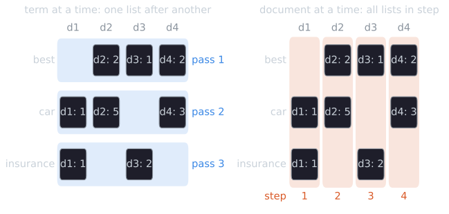
On the running example with $K = 2$, document-at-a-time evaluation proceeds as follows. At each step the cursors that point at the smallest docID advance together, and that document's score is complete.
| Step | Document | Postings read | Score | Heap action | Heap after (smallest first) |
|---|---|---|---|---|---|
| 1 | $d_1$ | car, insurance | 0.246 | push | $d_1$ 0.246 |
| 2 | $d_2$ | best, car | 0.159 | push | $d_2$ 0.159, $d_1$ 0.246 |
| 3 | $d_3$ | best, insurance | 0.234 | 0.234 > 0.159: replace $d_2$ | $d_3$ 0.234, $d_1$ 0.246 |
| 4 | $d_4$ | best, car | 0.118 | 0.118 < 0.234: discard | $d_3$ 0.234, $d_1$ 0.246 |
The answer is the same as term-at-a-time, as it must be. What differs is the state kept along the way: term-at-a-time held four accumulators before it could rank anything, while document-at-a-time never held more than two scored documents and three cursors. On a real collection the difference is between memory proportional to the number of matching documents and memory proportional to $K$.
The trace also shows where skipping comes from. When $d_4$ is reached, the heap's smallest score, 0.234, is the bar to clear. If the system knew in advance that no document lacking insurance can score above, say, 0.2, it could skip every such document without computing its score. MaxScore and WAND precompute, for each term, the largest contribution it can make to any document, and use these bounds to skip documents, or whole stretches of a postings list, that cannot clear the bar.
Shortcuts when exact scores cost too much
For very large collections, even the postings of a query's terms are too long to process completely. Manning, Raghavan, and Schütze (2008, §§7.1 and 7.2.1) describe heuristics that return the top $K$ documents approximately, accepting a small risk of missing one of the true top $K$ in exchange for much less work:
- Index elimination. Skip query terms with low IDF, like sale above, since their contributions are small and their postings lists long. Or consider only documents that contain several of the query terms.
- Champion lists. For each term, precompute a short list of the documents with the highest weights for it, and score only documents on the query terms' champion lists.
- Static quality ordering. Order postings by a query-independent quality score, such as PageRank, so that processing can stop early with good documents already found.
- Tiered indexes. Divide each postings list into tiers by term weight, for example documents in which the term occurs more than 20 times in the first tier, and consult lower tiers only if the first returns too few results.
Index elimination measured
How much does skipping low-IDF terms save, and what does it cost? On the Cranfield collection (1,400 abstracts, 225 queries with a median of 11 distinct terms after stop-word removal), lnc.ltc scoring term at a time creates a median of 1,027 accumulators per query, for nearly three-quarters of the collection, because Cranfield's queries are full sentences that contain common words of the field. Skipping query terms below an IDF threshold changes the picture as follows:
| Skip terms with IDF below | Median accumulators | Postings read (all queries) | Median overlap with exact top 10 | Mean average precision |
|---|---|---|---|---|
| none (exact) | 1,027 | 465,318 | 10 | 0.294 |
| 0.5 | 816 | 322,731 | 9 | 0.287 |
| 0.75 | 563 | 182,094 | 8 | 0.281 |
| 1.0 | 276 | 78,779 | 6 | 0.234 |
| 1.5 | 47 | 13,191 | 3 | 0.140 |
An IDF of 0.5 corresponds to a term in about a third of the documents, and 1.0 to one in a tenth. Skipping only the commonest terms cuts the postings read by about a third and costs little: nine of the ten top results are unchanged, and mean average precision falls by 0.007. Pushed further, the savings keep growing but the results degrade quickly, because terms that occur in a tenth of an abstract collection still carry much of a query's meaning. The right threshold is a trade-off measured on the collection at hand, which is why such shortcuts are tuned with evaluation rather than set by rule.
Ranking does not require exact scores, only the right order at the top. That is why approximate methods are acceptable in practice, and why exact methods such as WAND, which skip documents only when they provably cannot reach the top $K$, are often fast enough not to need them.
The running-example traces are computed by tools/experiments/vsm/running_example.py, the code blocks are run and checked by tools/experiments/vsm/check_cosine_score.py, the Cranfield measurements come from tools/experiments/vsm/cranfield_elimination.py (deterministic), and the figure from tools/figures/computing-vector-scores.py, all in the site repository.
References
- Manning, C. D., Raghavan, P., and Schütze, H. (2008). Introduction to Information Retrieval, sections 6.3.3, 7.1, and 7.2.1. Cambridge University Press.
- Turtle, H., and Flood, J. (1995). Query evaluation: Strategies and optimizations. Information Processing and Management, 31(6), 831–850.