Cosine similarity is symmetric: it compares any two vectors, not only a query with a document. Comparing documents with each other supports a range of tasks. It can find duplicates and near-duplicates, suggest related articles, offer a "more like this" link, and group documents for clustering. The most demanding form of the task is all-pairs similarity: find the $k$ most similar pairs of documents in an entire collection. That was the third assignment in the course, and this article uses my solution, HW03 on GitHub, to show why the problem is hard and how much the implementation matters.
Why all-pairs is quadratic
A collection of $N$ documents has $N(N-1)/2$ distinct pairs:
| Documents | Pairs |
|---|---|
| 1,000 | 499,500 |
| 5,000 | 12,497,500 |
| 30,000 | 449,985,000 |
| 1,000,000 | about $5 \times 10^{11}$ |
Each comparison is a cosine similarity between two sparse vectors. Multiplying the collection size by 30 multiplies the number of pairs by about 900. No amount of constant-factor optimization changes that growth, so the practical questions are how small the constant can be made, and how many of the pairs can be skipped without computing them.
The assignment
HW03 asked for the most similar document pairs in a collection under three weighting schemes:
- tf: raw term frequency;
- tf-idf: term frequency times $\log_{10}(N/\mathit{df})$, as in TF-IDF weighting;
- wf-idf: sublinear term frequency $1 + \log_{10} \mathit{tf}$ times the same IDF, as in variants of TF-IDF.
Each document's vector is weighted and its length precomputed once, so each comparison reduces to a dot product over the terms the two documents share, divided by the two stored lengths.
I wrote three implementations behind a common interface, with a factory that chooses among them at run time (see designing a modular search engine):
- Standard: a single-process loop over the upper triangle of the pair matrix. Each document is stored as a dictionary of term weights. For each pair, the code intersects the two dictionaries' keys, skips pairs with no common terms, computes the dot product over the shared terms, and keeps the best $k$ pairs in a min-heap.
- Parallel: the same computation divided into tiles, each covering a block of documents compared against another block. Each task copies its blocks' weight vectors to a worker process, the worker returns every pair with nonzero similarity, and the parent process selects the top $k$ with a heap.
- Sparse: the weighted collection as a sparse matrix in compressed sparse row (CSR) format, with all pairwise cosines computed at once by scikit-learn's
cosine_similarity, and the top $k$ selected with NumPy'sargpartition, which finds the largest values without fully sorting.
Benchmarks
I measured all three on collections of increasing size, on my own machine. Times are in seconds. Because the program computes all three weighting schemes on every run, each time covers three all-pairs passes plus building the model:
| Documents | Standard | Parallel | Sparse |
|---|---|---|---|
| 1,000 | 2.84 | 11.96 | 1.01 |
| 2,000 | 9.90 | 15.17 | 1.99 |
| 3,000 | 18.52 | 18.06 | 3.00 |
| 4,000 | 31.82 | 22.33 | 4.07 |
| 5,000 | 48.57 | 25.76 | 4.97 |
| 15,000 | 449.50 | 101.26 | 20.97 |
| 30,000 | 1,928.29 | 368.93 | 55.89 |
The quadratic growth is visible. From 1,000 to 30,000 documents, the standard implementation's time grew by a factor of 679, approaching the factor of 901 in the number of pairs.
Parallelism has a fixed cost. Starting worker processes, copying weight vectors to them, and returning every nonzero pair to the parent costs several seconds, so the parallel version was four times slower than the standard one at 1,000 documents. The two crossed between 2,000 and 3,000 documents, and beyond that parallelism paid off, reaching a fivefold speedup at 30,000. The factory's threshold of 2,500 documents for choosing the parallel version came from this measurement.
Sparse matrices win twice. The sparse implementation, running in a single process, was the fastest at every size, by a factor of 35 over the standard version at 30,000 documents and nearly 7 over the parallel one. Part of the advantage is that its arithmetic runs in compiled routines rather than a Python loop. The other part is that it does less work. Multiplying the weighted document matrix by its transpose only combines documents that share a term, so pairs with nothing in common are never visited. That is the inverted-index strategy described below, carried out by a sparse-matrix library.
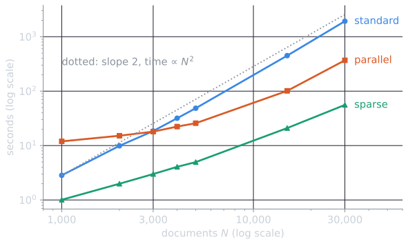
Logarithmic axes turn the question "how fast does the cost grow?" into "how steep is the line?". If time is $c N^a$, then $\log(\text{time}) = \log c + a \log N$, a straight line of slope $a$. Over the three largest sizes, the slopes are 2.05 for the standard implementation, 1.46 for the parallel one and 1.35 for the sparse one. The standard implementation is in the quadratic regime already. The other two grow more slowly over this range, presumably because part of their time goes to work that grows roughly linearly with $N$, such as building the weighted vectors and starting workers, and because pairs with no shared term cost the sparse product nothing. As $N$ grows, the quadratic part must eventually dominate, and their slopes should approach 2 as well.
The memory wall
The sparse implementation computes the entire similarity matrix at once. Its time is excellent, but its memory grows with the number of document pairs that share at least one term. In a collection where common words survive stop-word removal, a large fraction of pairs share some term, so the "sparse" result can be nearly dense. In the 10,788 news stories of Reuters-21578, 84% of the 58 million pairs share at least one word even after a 33-word stop list is removed, because words such as said occur in most stories (measurements below). At 30,000 documents, a dense matrix of 4-byte floats would need 3.6 gigabytes, and a nearly full sparse matrix would need more, since it stores an index alongside each value. At a million documents the dense matrix would need 4 terabytes. The time cost is quadratic, and so, unless the computation is restructured, is the memory cost. The standard remedy is to process the matrix in blocks of rows, keeping only each block's best candidates before moving on, which preserves the speed of vectorized code while bounding memory.
Skipping pairs with the inverted index
The standard and parallel implementations consider every pair, even pairs that share no terms and whose similarity is therefore zero. They check for shared terms before computing anything, but the check itself is made for every pair. The inverted index lets an algorithm touch only pairs that share a term. Treat each document in turn as a query, and accumulate dot products from the postings lists of its terms, exactly as in computing vector scores. Every pair that shares no term is never visited.
The work then depends on the postings lists rather than on $N^2$. A term with document frequency $\mathit{df}_t$ contributes a partial product to each of the roughly $\mathit{df}_t^2 / 2$ pairs of documents containing it. Rare terms cost almost nothing, while a very common term costs nearly as much as the full quadratic computation. Since common terms also have low IDF and contribute little to similarity, practical systems drop or down-weight them, accepting slightly approximate scores in exchange for a large saving.
Counting the work
The running example of this topic (four documents, introduced in TF-IDF weighting) shows the accounting on a small scale. Its postings lists have document frequencies 2 (auto), 3 (best), 3 (car), 2 (insurance), 1 (loan) and 2 (rate), so the terms generate $1 + 3 + 3 + 1 + 0 + 1 = 9$ partial products, one for each pair of documents within each list. There are only $4 \times 3 / 2 = 6$ pairs, and every one of them shares at least one term, so the inverted-index method skips nothing here and does more multiplications than comparing every pair would. A pair that shares $m$ terms receives $m$ partial products, one from each shared term's list.
On a real collection the balance depends on the common terms. The table counts, for all 10,788 documents of Reuters-21578 (words lowercased, no stemming), the pairs that share at least one word and the partial products the inverted-index method would compute, $\sum_t \mathit{df}_t(\mathit{df}_t - 1)/2$:
| Terms indexed | Pairs sharing a term | Partial products | Products per pair |
|---|---|---|---|
| all words | 90.0% | 492.6 million | 8.47 |
| 33-word stop list removed | 84.2% | 254.9 million | 4.38 |
| also words in more than 10% of documents (60 words) | 42.0% | 68.4 million | 1.18 |
| also words in more than 5% of documents (197 words) | 25.3% | 31.8 million | 0.55 |
"Products per pair" divides the partial products by all 58,185,078 pairs. With every word indexed, the inverted-index method skips only the 10% of pairs that share nothing, and it computes more than eight partial products for every pair in the collection, because nearly every pair shares of, the or to and each shared word adds a product. Removing the stop list halves that, and said (in 6,784 of the 10,788 stories) becomes the commonest term. Dropping the 197 words that occur in more than 5% of the stories, under 1% of the vocabulary of about 29,000 words, cuts the products by a factor of eight more, and three-quarters of all pairs are then never touched. The saving that makes the inverted-index method fast comes from setting aside a small number of very common terms, and the cost is that similarities are computed without them.
When only pairs above a similarity threshold are wanted, much more can be skipped. Bayardo, Ma, and Srikant (2007) showed how to index only part of each vector, the part needed to guarantee that any pair above the threshold is found, so that most low-similarity pairs are never considered. Their method computes the exact answer far faster than examining all pairs.
Approximate methods
For web-scale collections, even these methods are too slow, and systems accept approximate answers. Locality-sensitive hashing assigns each document short signatures chosen so that similar documents are likely to share them. Candidate pairs are then only those that share a signature, and only they are compared exactly. MinHash signatures estimate the overlap between documents' sets of word sequences, the basis of near-duplicate detection on the web (Broder, 1997). Random-projection signatures estimate cosine similarity directly (Charikar, 2002). Both reduce the problem from all pairs to the few pairs that matter.
What the weighting changes
The three weighting schemes find different "most similar" pairs. With raw term frequency, documents that share heavily repeated common terms look similar regardless of subject. IDF reduces the influence of terms that appear everywhere, so pairs are matched on distinctive vocabulary. Sublinear weighting further reduces the influence of any one repeated term.
The running example shows all three effects on its six pairs. The cosines below use the three HW03 schemes, each with cosine normalization (nnc, ntc and ltc in the SMART notation of variants of TF-IDF), rounded to three decimals:
| Pair | tf | tf-idf | wf-idf |
|---|---|---|---|
| $d_1$, $d_2$ (headline, car review) | 0.527 | 0.239 | 0.148 |
| $d_1$, $d_3$ (headline, auto insurance) | 0.309 | 0.374 | 0.439 |
| $d_1$, $d_4$ (headline, car loans) | 0.562 | 0.275 | 0.324 |
| $d_2$, $d_3$ (car review, auto insurance) | 0.244 | 0.376 | 0.632 |
| $d_2$, $d_4$ (car review, car loans) | 0.563 | 0.154 | 0.149 |
| $d_3$, $d_4$ (auto insurance, car loans) | 0.087 | 0.011 | 0.031 |
With raw counts, the most similar pair is the car review and the car-loan page, which share the repeated words car and best, and the three pairs involving car fill the top. IDF demotes car and best, which are in three of the four documents, and the pairs linked by rarer words rise: the headline and the auto-insurance page share insurance, and the car review and the auto-insurance page share auto. Sublinear weighting then reduces the car review's five occurrences of car, which makes its vector point more toward auto and best, and the review and the auto-insurance page become the clear top pair. That is a reminder of what these measures see. The two documents are not about the same thing; they share two words, one of them rare in this collection, and nothing in the vectors records that one page is about buying a car and the other about insuring one.
In a collection containing exact or near duplicates, those pairs rank at the top under every scheme, with cosine values at or near 1, which is why duplicate detection is often the first practical use of an all-pairs comparison.
The running-example cosines and pair counts are computed by tools/experiments/vsm/running_example.py, the Reuters counts by tools/experiments/vsm/reuters_pairs.py (exact, no sampling), and the figure by tools/figures/document-similarity.py, all in the site repository.
References
- Bayardo, R. J., Ma, Y., and Srikant, R. (2007). Scaling up all pairs similarity search. In Proceedings of WWW 2007, 131–140.
- Broder, A. Z. (1997). On the resemblance and containment of documents. In Proceedings of Compression and Complexity of Sequences 1997, 21–29.
- Charikar, M. S. (2002). Similarity estimation techniques from rounding algorithms. In Proceedings of STOC 2002, 380–388.
- Manning, C. D., Raghavan, P., and Schütze, H. (2008). Introduction to Information Retrieval, sections 6.3 and 19.6. Cambridge University Press.