The third assignment in CSC 742 set a bin packing problem in the language of an online shop. Orders weighing between 0 and 2 kg each are to be packed into boxes that hold at most 10 kg, using as few boxes as possible. The assignment fixed most of the design. An individual is a list of integers, one per item, giving the bin that item goes into, with bin labels from 0 to $N - 1$ for $N$ items. Two quantities are computed for each individual: $f$, the number of distinct bins used, and $g$, the number of bins whose load exceeds the capacity. Parents are chosen by binary tournaments with feasibility-first rules, followed by one- or two-point crossover and a mutation that reassigns a gene to a random bin. The GA was to run with a population of 20 for 50 generations on 10, 25, 50 and 100 items, with variations in population size and run length.
This article reports what I submitted, explains why it stopped far from the optimum, and compares it with a classical heuristic, a lower bound, and a different encoding. The experiment script is tools/experiments/evolution/bin_packing.py in the site repository; the figures and the small worked examples come from tools/figures/genetic-algorithm-bin-packing.py.
The submitted algorithm
The program (bpp_ga.py) followed the specification closely. Initial genes were uniform on $0, \dots, N - 1$. The tournament compared two random individuals by three rules: if both are feasible ($g = 0$), the one with fewer bins wins; if only one is feasible, it wins; if neither is, the one with fewer overfull bins wins. These are the tournament rules Deb (2000) proposed for constrained optimization, with the number of violated bins standing in for his total amount of violation. One tournament per member of the population filled a mating pool, from which pairs were drawn at random. Two-point crossover was applied with probability 0.9, and each gene was reset to a uniformly random bin label with probability $1/N$. Offspring replaced the population, with no elitism, and the best individual ever evaluated was reported.
The program seeded Python's random number generator once per pass (seeds 42, 773 and 2025), then generated a fresh set of item weights for every combination of configuration and size, drawing from the same stream. Rerunning the same call sequence with seed 42 reproduces every number the report gave:
| Configuration | 10 items | 25 items | 50 items | 100 items |
|---|---|---|---|---|
| Baseline (pop 20, 50 generations) | 3 | 7 | 18 | 42 |
| Small population (pop 10) | 2 | 8 | 20 | 43 |
| Large population (pop 40) | 2 | 7 | 18 | 37 |
| Short run (25 generations) | 3 | 9 | 22 | 52 |
| Long run (100 generations) | 2 | 8 | 17 | 37 |
The report observed that every run had feasible individuals from generation 0, and concluded that the constraint rules, though implemented, were never needed. The rerun confirms that they had almost nothing to do: of the 24,000 individuals evaluated at seed 42, 4 had an overfull bin. It concluded that larger populations and longer runs both helped, most of all on 100 items, and that the search settled in local optima made of many partly filled bins. It noted that the best packings used "nearly 4x more bins than necessary", with most bins holding only 2 to 4 kg, and traced the gap to operators that make incremental improvements but "struggle to discover the coordinated item rearrangements needed for dense packing". The sections below take that observation further.
How far from optimal
The simplest lower bound on the number of bins is the total weight divided by the capacity, rounded up (Martello and Toth, 1990, §8.3.1):
$$L_1 = \left\lceil \frac{\sum_{i=1}^{N} w_i}{C} \right\rceil.$$
An upper bound comes from First Fit Decreasing (FFD): sort the items from heaviest to lightest, and put each into the first bin, in order of opening, that still has room, opening a new bin when none does. Johnson (1973) proved that FFD never uses more than $\frac{11}{9}\mathrm{OPT} + 4$ bins, where OPT is the optimum, and Dósa (2007) lowered the additive constant to the best possible value:
$$\mathrm{FFD}(I) \le \tfrac{11}{9}\,\mathrm{OPT}(I) + \tfrac{6}{9}.$$
A small instance shows how the bound and first fit work, and why the order of the items matters. Take eight items A to H weighing 6, 5, 5, 4, 4, 3, 2 and 1 kg, and boxes of 10 kg. The total is 30 kg, so $L_1 = \lceil 30 / 10 \rceil = 3$: no packing can use fewer than three bins, and a three-bin packing must fill every bin exactly. First fit in decreasing order places the items like this:
| Item | Weight | Placed in | Bin loads afterwards |
|---|---|---|---|
| A | 6 | bin 1 (new) | 6 |
| B | 5 | bin 2 (new; does not fit in bin 1) | 6, 5 |
| C | 5 | bin 2 | 6, 10 |
| D | 4 | bin 1 | 10, 10 |
| E | 4 | bin 3 (new) | 10, 10, 4 |
| F | 3 | bin 3 | 10, 10, 7 |
| G | 2 | bin 3 | 10, 10, 9 |
| H | 1 | bin 3 | 10, 10, 10 |
Three bins, equal to $L_1$, so this packing is optimal. The same rule applied in increasing order, H first, fills bin 1 with H, G, F and E (1 + 2 + 3 + 4 = 10), puts D and C in bin 2 (9 kg), and then has no room for B or A anywhere: B opens bin 3, and A, at 6 kg, does not fit with B and opens bin 4. Four bins.
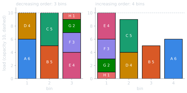
Large items placed first leave the small ones to fill the gaps; small items placed first use up the space that the large ones needed. That is the reasoning behind sorting before packing, and it is also why an encoding that chooses the order, as the one later in this article does, can reach good packings with a simple decoder.
When FFD and $L_1$ agree, both equal the optimum. On the twenty instances of the submission, they agree on nineteen. For the baseline instances, the optimum is 2, 3, 6 and 11 bins, against the GA's 3, 7, 18 and 42; the report's estimate of "approximately 10" for 100 items was close but the optimum is 11. The ratio to the optimum grows with the problem: 1.5, 2.3, 3.0 and 3.8. The single exception is the short run's 100-item instance, whose weights total 99.98 kg, so that $L_1 = 10$ while FFD uses 11. Ten bins would have only 0.024 kg of free space among them, and neither bound settles whether such a packing exists.
The same check shows something that a table of single runs cannot. Because every configuration drew its own weights, each row of the table above was run on different instances. The large-population and long-run configurations both reached 37 bins on 100 items, but against optima of 10 and 12. Differences between rows mix the effect of the parameters with the luck of the instance, and with one seed per row the two cannot be separated.
Thirty seeds on fixed instances
To separate them, the script fixes the four baseline instances and reruns the submitted GA with seeds 0 to 29 at the same budget of 20 individuals for 50 generations, 1,000 evaluations in all:
| Items | Total weight | $L_1$ = FFD = OPT | Assignment GA, median [IQR] | Range |
|---|---|---|---|---|
| 10 | 10.47 kg | 2 | 2 [2, 3] | 2 to 3 |
| 25 | 27.49 kg | 3 | 8 [7, 8] | 6 to 9 |
| 50 | 55.10 kg | 6 | 17.5 [17, 19] | 15 to 20 |
| 100 | 101.24 kg | 11 | 42 [41, 43] | 38 to 47 |
The baseline's single results (3, 7, 18, 42) are typical of the distribution. More computation helps, slowly.
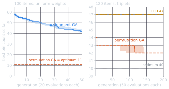
The left panel shows the shape of the assignment GA's progress on 100 items: medians of 58 bins after the first generation, 53 after 10, 48 after 25 and 42 after 50, about one bin every three generations with no sign of levelling off. The runs were stopped, not converged. On the 100-item instance the median falls to 33 bins with a population of 40 for 100 generations, and to 20 bins with a population of 100 for 500 generations, fifty times the original budget, which is still nearly twice the optimum.
Why the assignment encoding struggles
What a stalled run looks like is clearest on the 25-item instance. The run with seed 0 ended with 7 bins, against an optimum of 3:
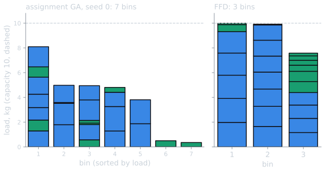
The GA's bins hold 8.10, 4.98, 4.95, 4.81, 3.81, 0.50 and 0.35 kg. The last two each contain one light item, and emptying either would save a bin, but nothing in the search rewards moving a 0.35 kg item into a bin that has room for it until the move is made, and a random reset of that one gene is far more likely to open a new bin than to pick one of the six labels in use. The paragraphs below take these effects one at a time.
The encoding is highly redundant. Bin labels carry no meaning, so any packing can be written under many relabelings. A packing of 100 items into 11 bins, with labels drawn from 0 to 99, has $100 \times 99 \times \dots \times 90 \approx 5.7 \times 10^{21}$ encodings. Two parents that contain the same good bin under different labels cannot pass it on together: two-point crossover copies a stretch of labels from one parent into the other, and the copied labels mean different bins in the receiving parent. What crossover transmits is "item 17 is in bin 4", a fact whose meaning depends on where the rest of bin 4 sits in the same chromosome, rather than "items 17, 23 and 61 belong together", which is the information a good packing contains. This is the motivation for representations in which the bins themselves are the units of inheritance.
The eight-item example makes this concrete. Both parents below describe the same optimal packing, {A, D}, {B, C} and {E, F, G, H}, each bin holding exactly 10 kg, under different labels. Gene $i$ is the label of item $i$'s bin, in the order A to H. Two-point crossover with cuts after positions 2 and 5 swaps the genes of C, D and E:
| A | B | C | D | E | F | G | H | |
|---|---|---|---|---|---|---|---|---|
| Parent 1 | 0 | 1 | 1 | 0 | 2 | 2 | 2 | 2 |
| Parent 2 | 5 | 0 | 0 | 5 | 3 | 3 | 3 | 3 |
| Child 1 | 0 | 1 | 0 | 5 | 3 | 2 | 2 | 2 |
| Child 2 | 5 | 0 | 1 | 0 | 2 | 3 | 3 | 3 |
Grouping the items by label gives the bins, written as label: items (load in kg):
- Parent 1: 0: AD (10), 1: BC (10), 2: EFGH (10).
- Parent 2: 5: AD (10), 0: BC (10), 3: EFGH (10).
- Child 1: 0: AC (11, overfull), 1: B (5), 5: D (4), 3: E (4), 2: FGH (6).
- Child 2: 5: A (6), 0: BD (9), 1: C (5), 2: E (4), 3: FGH (6).
Two optimal, identical packings produce children with five bins each, one of them infeasible. Label 0 means "the bin of A and D" in parent 1 and "the bin of B and C" in parent 2, so copying C's label from parent 2 into parent 1 sends C to A's bin. With a permutation of the items and a decoder, two parents that are the same packing in the same order produce that packing again.
The objective gives almost no guidance. The fitness is the number of distinct labels. It falls by one only when a bin is emptied completely, and a bin of three items is emptied only if all three move elsewhere. Partial progress, such as moving two of the three, scores exactly the same as no progress, so selection cannot reward it.
Mutation mostly opens new bins. A reset gene takes a uniformly random label from 0 to $N - 1$. When a 100-item individual uses 42 labels, the new label is one of the 58 unused ones with probability 0.58, and the item moves to a bin of its own. Random initialization starts high for the same reason: $N$ items placed independently into $N$ bins occupy $N(1 - (1 - 1/N)^N)$ bins on average, about 63 for $N = 100$. The search starts far from the optimum and its main operator pushes back toward where it started.
The capacity constraint rarely binds. With items averaging 1 kg, a bin overflows only when it holds at least six items. Random assignments almost never put that many together, and selection pressure pushes toward fewer bins only slowly, so almost every individual the GA evaluated was feasible. The constraint-handling machinery, which the assignment emphasized, played almost no part. That was a property of the instances, which the report recognized, not a sign that the problem was easy for this encoding.
A permutation encoding with a decoder
An alternative representation encodes an order of the items and leaves the packing to a deterministic decoder, here first fit: take the items in the encoded order and put each into the lowest-numbered bin that has room, opening a new bin when none has. Every permutation decodes to a feasible packing, so the constraint disappears from the search, which is the idea behind decoder-based constraint handling (Eiben and Smith, 2015, ch. 13; see constraint handling in evolutionary algorithms).
Nothing is lost by restricting the search to first-fit packings. Take any packing into $k$ bins and list its items bin by bin. Decoding that order with first fit uses at most $k$ bins: the items of each listed bin either fit into bins already open or go into new ones, and they can open at most one new bin between them, since their total weight fits in one bin and a newly opened bin holds only items of the current group. So some order decodes to an optimal packing.
The permutation GA in the script uses binary tournaments, order crossover with probability 0.9, and swap mutation in which each position is swapped with a random position with probability $1/N$ (Eiben and Smith, 2015, ch. 4, describe these operators for permutations). It keeps one elite individual. The fitness is compared lexicographically: first the number of bins, then, among packings with equally many bins, the larger value of $\sum_j (\ell_j / C)^2$, where $\ell_j$ is the load of bin $j$. The second term favors packings that concentrate the load in some bins and leave others nearly empty, which is the partial progress the bare bin count cannot see.
With the same budget of 1,000 evaluations, on the same four instances and the same thirty seeds, the permutation GA reached the optimum in every run, 2, 3, 6 and 11 bins. So did a control with no evolution at all: the best of 1,000 random orders, each decoded by first fit. On these instances the decoder does the work. When first fit opens a new bin for an item of at most 2 kg, every bin already open holds more than 8 kg, so in any order all bins but the last are more than 80 percent full. For the 100-item instance that limits any order to at most 13 bins. In fact, of 10,000 random orders, every one decodes to an optimal packing on each of the four instances. The assignment's instances turn out to be easy; the difficulty the GA met came from the integer encoding.
Harder instances
The instance class matters more than the parameter settings. Falkenauer contributed a family of hard test instances to OR-Library (Beasley, 1990), the triplets, built with a known optimum of $N/3$ bins, three items to a bin. The script generates instances in the same style: for each triplet it draws a first item of 380 to 490 units, a second of 250 units up to half the remainder, and a third that fills the bin of capacity 1,000 exactly, then shuffles all the items together. The total weight is then exactly $N/3$ full bins, so any packing that leaves space unused in even one bin needs an extra bin.
| Items | OPT | FFD | Permutation GA, 10,000 evaluations, median [IQR] | Runs at OPT |
|---|---|---|---|---|
| 60 | 20 | 24 | 21 [21, 21] | 0 of 30 |
| 120 | 40 | 47 | 42 [42, 42] | 0 of 30 |
Here FFD is far from the optimum, the permutation GA improves on it substantially, and neither reaches the optimum in any run. On the 120-item instance the best of the GA's 50 random initial orders already gives a median of 44 bins, three fewer than FFD; evolution then gains two more bins over 200 generations, most of the way in two steps (the right panel of the convergence figure above). Falkenauer's (1996) grouping genetic algorithm was designed for problems of this kind: a GA "heavily modified to suit the structure of grouping problems", in which the genes represent groups, here bins, so that the operators can pass on whole bins. He combined it with a local optimization inspired by the dominance criterion of Martello and Toth, and reports that the combination outperformed both of its components. Building that representation is the natural next step for this experiment.
Lessons
- Compare with a baseline and a bound before tuning. A two-line FFD and the bound $L_1$ show at once that the optimum is 11 bins, and so that the GA's 42 reflects the method rather than the problem.
- Hold the instance fixed when comparing parameter settings, and run each setting over many seeds.
- Choose a representation in which the units of a good solution can be inherited. For bin packing those units are groups of items, which neither the item-to-label encoding nor the bare bin count represents.
- Give selection a gradient. A fitness that changes only when a bin empties cannot reward the steps that lead there.
- Test on instances that can tell methods apart. On the assignment's instances, random orders with a good decoder were already optimal.
References
- Beasley, J. E. (1990). OR-Library: distributing test problems by electronic mail. Journal of the Operational Research Society, 41(11), 1069–1072.
- Deb, K. (2000). An efficient constraint handling method for genetic algorithms. Computer Methods in Applied Mechanics and Engineering, 186(2–4), 311–338.
- Dósa, G. (2007). The tight bound of First Fit Decreasing bin-packing algorithm is FFD(I) ≤ 11/9 OPT(I) + 6/9. In Combinatorics, Algorithms, Probabilistic and Experimental Methodologies (ESCAPE 2007), Lecture Notes in Computer Science 4614, 1–11. Springer.
- Eiben, A. E., and Smith, J. E. (2015). Introduction to Evolutionary Computing, 2nd ed., chapters 4 and 13. Springer.
- Falkenauer, E. (1996). A hybrid grouping genetic algorithm for bin packing. Journal of Heuristics, 2(1), 5–30.
- Johnson, D. S. (1973). Near-Optimal Bin Packing Algorithms. PhD thesis, Massachusetts Institute of Technology.
- Martello, S., and Toth, P. (1990). Knapsack Problems: Algorithms and Computer Implementations, chapter 8. Wiley.