In March 2006 three small NASA spacecraft were launched carrying an X-band antenna that no engineer had drawn. It was a bent wire of irregular shape, small enough to fit in a cylinder 15 cm across, and it had been found by an evolutionary algorithm searching a space of wire shapes, each one scored by an electromagnetic simulator. The antenna is the best-known evolved artifact in engineering, but it is not the only one. This article describes several cases in which evolutionary search produced designs that were built, tested or used, says precisely what each showed, and then considers where evolutionary methods sit among the optimization tools engineers actually use.
The ST5 antenna
NASA's Space Technology 5 (ST5) mission flew three micro-satellites, each about 53 cm across and 25 kg when fueled, to test new technologies while measuring the magnetosphere. Each carried two antennas, one on top and one on the bottom. The original requirements, for a highly elliptical orbit, asked for a right-hand circularly polarized gain of at least 0 dBic at angles θ from 40° to 80° in every azimuth (Hornby and colleagues write θ and call these angles elevations; their statement below, that the four-arm design has a null at the zenith that rules it out for the new requirement at small θ, indicates that θ is measured from the zenith, so θ = 0° points straight up), a voltage standing wave ratio (VSWR) below 1.2 at the transmit frequency of 8470 MHz and below 1.5 at the receive frequency of 7209.125 MHz, a 50-ohm input impedance, a mass under 165 g, and a fit inside a cylinder 15.24 cm in diameter and height (Hornby, Globus, Linden, and Lohn, 2006).
The team did not let evolution search all possible antennas. Engineers chose the class first: monopole wire antennas. Two evolutionary algorithms were used, one with a fixed-length vector of real-valued parameters and one with a tree-structured generative representation, in which each node is a construction operator such as "add a wire of this length" or "rotate by this angle about an axis", and executing the tree draws the antenna (Hornby, Lohn, and Linden, 2011). For the original requirements the search was restricted to four identical arms, each rotated 90° from its neighbors, so that only one arm had to be evolved. Fitness multiplied three penalty terms, for VSWR, for gain error, and for the number of sampled directions in which gain fell below the minimum, and the algorithm minimized the product. The best design, ST5-3-10, met the requirements and was on track to fly.
Then the launch vehicle changed, putting the spacecraft in a much lower orbit and adding a requirement of at least −5 dBic at θ from 0° to 40°, the cone around the zenith. The four-arm symmetric design has a null at the zenith, so the team changed the representation to a single, non-branching arm (branching designs had also proved hard to fabricate precisely), replaced the outlier term with one that rewarded a gain pattern smooth in azimuth, since the spacecraft spin at about 40 revolutions per minute, and rewrote the gain penalty with separate targets and weights for each elevation band. In less than a month they evolved a new design, ST5-33-142-7, whose compliance was confirmed in an anechoic chamber at NASA Goddard Space Flight Center. It flew on the mission launched on 22 March 2006, and the designers describe it as the first computer-evolved antenna deployed for any application (Hornby, Globus, Linden, and Lohn, 2006; Hornby, Lohn, and Linden, 2011).
The design problem in numbers
Set side by side, the requirements show how much of the problem was fixed before evolution started (Hornby, Globus, Linden, and Lohn, 2006, §II):
| Requirement | Original orbit | After the orbit changed |
|---|---|---|
| Gain, right-hand circular polarization | ≥ 0 dBic for 40° ≤ θ ≤ 80°, all azimuths | also ≥ −5 dBic for 0° ≤ θ ≤ 40° |
| VSWR at the transmit frequency, 8470 MHz | < 1.2 | unchanged |
| VSWR at the receive frequency, 7209.125 MHz | < 1.5 | unchanged |
| Input impedance | 50 Ω at both frequencies | unchanged |
| Mass | < 165 g | unchanged |
| Size | inside a cylinder 15.24 cm in diameter and height | unchanged |
| Antenna class searched | monopole wire, four identical arms 90° apart | monopole wire, one non-branching arm |
| Fitness, minimized | VSWR term × gain-error term × outlier count | VSWR term × gain-error term × smoothness term |
The table separates what the engineers decided from what evolution decided. The frequencies, impedance, mass and envelope came from the mission; the antenna class, the symmetry and the form of the fitness function came from the antenna designers; only the shape of the wire inside those limits came from search.
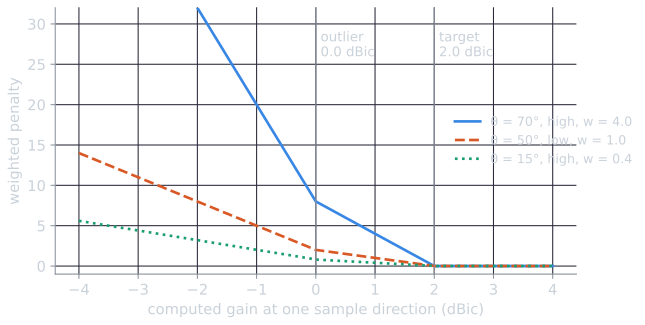
The revised gain term shows how engineering judgement was written into the fitness function. Gain was computed every 5° in θ and in azimuth $\phi$. For the elevation index $i$ (so $\theta = 5i°$, $i = 0, \dots, 18$) and a computed gain $g$ at one sample direction, the paper gives the penalty as (Hornby, Globus, Linden, and Lohn, 2006, §II.B)
$$\text{penalty}_i(g) = w_i \times \begin{cases} 0 & g \ge t_i, \\ t_i - g & o_i \le g < t_i, \\ (t_i - o_i) + 3\,(o_i - g) & g < o_i, \end{cases}$$
where $t_i$ is a target gain and $o_i$ an outlier level below it. For $i = 0$ to 16 ($\theta$ up to 80°), $t_i = 2.0$ dBic and $o_i = 0.0$ dBic; for $i = 17$ and 18 ($\theta = 85°$ and 90°, near the horizon on that reading of θ), $t_i = -3.0$ and $o_i = -5.0$. The target sits 2 dB above the original 0 dBic requirement, so a design is pushed to keep a margin, and below the outlier level the penalty grows three times as fast, so a single deep gap costs more than a uniform shortfall of the same total. The weights $w_i$ differ by band and by angle:
| θ (index $i$) | Weight, low band | Weight, high band |
|---|---|---|
| 0° to 35° (0 to 7) | 0.1 | 0.4 |
| 40° to 60° (8 to 12) | 1.0 | 3.0 |
| 65° (13) | 1.0 | 3.5 |
| 70° (14) | 1.0 | 4.0 |
| 75° (15) | 1.0 | 3.5 |
| 80° (16) | 1.0 | 3.0 |
| 85° and 90° (17, 18) | 0.05 | 0.2 |
The heaviest weights fall on 40° to 80°, the band of the original requirement, and peak at 70° in the high band. The gain term of the fitness is the sum of these penalties over all sampled directions.
A worked case: at θ = 70° in the high band ($w = 4.0$), a computed gain of 2.5 dBic costs nothing; 1.0 dBic meets the 0 dBic requirement but misses the target, and costs $4.0 \times (2.0 - 1.0) = 4.0$; −1.0 dBic violates the requirement and costs $4.0 \times ((2.0 - 0.0) + 3 \times (0.0 + 1.0)) = 20.0$. The same −1.0 dBic at θ = 85° in the high band costs nothing, because there the target is −3.0 dBic. These values are computed by tools/figures/evolved-designs-in-engineering.py.
The third term changed for a physical reason. The spacecraft spin at about 40 revolutions per minute, so a gain pattern that varies around the azimuth produces a signal that fluctuates with every turn. The smoothness term is a weighted sum, over elevations, of the standard deviation of the gain around the azimuth, using the same weights as the gain penalty (Hornby, Globus, Linden, and Lohn, 2006, §II.B). The VSWR term was kept from the original system. It applies strong pressure while the VSWR is above the required 1.2 (transmit) and 1.5 (receive), reduced pressure below 1.15 and 1.25, and no pressure to go below 1.1 (Hornby, Globus, Linden, and Lohn, 2006, §II.A). That graded shape, like the target and outlier levels of the gain term, encodes the designers' view of how much margin is worth having, and the fitness function, not the search algorithm, is the part of the system the authors changed when the requirements changed.
The comparison with the conventional design is part of the record. The mission had hired a contractor, who produced a quadrifilar helix antenna. On a spacecraft mock-up, two contractor antennas achieved 38% efficiency, one of each achieved 80%, and two evolved antennas achieved 93%; the evolved antenna needed no phasing circuit, and it took about three person-months to design and fabricate against about five for the conventional one. The authors attribute the speed of the redesign to "minimal changes" to their evolutionary system, "mostly in the fitness function" (Hornby, Globus, Linden, and Lohn, 2006). The limits of the evolutionary metaphor uses the same project to make that point about where engineering knowledge lives.
Satellite booms with unusual geometry
Keane (1995) applied a genetic algorithm to a problem in passive vibration control. A truss built from beams, of the kind used for satellite booms, transmits vibration from one end to the other, which matters when sensitive instruments sit at the far end. Engineers usually build such trusses from a regular, repeating geometry. Keane let a genetic algorithm move the joints of a two-dimensional truss, scoring each design by the band-averaged vibrational energy transmitted along it, computed with a purpose-built energy-flow analysis. The optimized geometry was irregular, unlike a standard truss. Keane's summary of the project gives the scale of the predicted effect: for a two-dimensional truss of 40 beams, 4,500 design evaluations over 18 generations reduced the predicted vibrational energy transmission by 60 dB over a 100 Hz band (Keane, n.d.).
The design was then built. Keane and Bright (1996) tested scale models of the optimized and the regular structures and reported that the models behaved somewhat differently from the predictions but showed the same broadband vibration isolation in practice. Keane and Brown (1996) extended the method to a three-dimensional boom, again starting from a regular repeating design and letting the genetic algorithm change the three-dimensional coordinates of its joints to minimize band-averaged noise transmission. According to Keane's summary of the project, the improvements came from geometry alone, with no weight penalty and only passive means, and the price was a structure that would be harder to build and deploy in space than a conventional one (Keane, n.d.).
An evolved circuit that used the physics of its chip
Thompson (1997) evolved a circuit directly on a reconfigurable chip, an approach he called intrinsic hardware evolution: every fitness evaluation configured a real field-programmable gate array (FPGA) and measured what it did. The chip was a Xilinx XC6216, of which a 10 × 10 corner of the 64 × 64 array of cells was used, configured by an 1800-bit genome. The task was to distinguish square waves of about 1 kHz and 10 kHz, outputting a steady high voltage for one and low for the other, with no clock and no external components. Each cell switches in a few nanoseconds, so the circuit had to discriminate periods five orders of magnitude longer than its own delays, and many people, Thompson wrote, thought this impossible.
The algorithm was an ordinary generational genetic algorithm: population 50, elitism, linear rank-based selection, single-point crossover with probability 0.7, and per-bit mutation set to give an expected 2.7 mutations per genome. Fitness was measured with an analog integrator over five 500 ms bursts of each tone in random order, as the difference between the average output voltages for the two tones. An earlier fitness that checked only whether the output was above or below the logic threshold had failed; the graded measure gave evolution a path of small improvements. Behavior that looked perfect on an oscilloscope appeared at about generation 3,500, the last glitches disappeared at about generation 4,100, and the run continued to generation 5,000 without visible change.
The finished circuit is the reason the experiment is remembered. A search for the largest set of cells that could be clamped to constant values without changing the behavior left a functional core of only 32 of the 100 cells. Some of those 32 had no connected path to the output, yet clamping them degraded performance, so they must have influenced the circuit through some route other than the normal wiring, probably the power supply or electromagnetic coupling between neighbors. The circuit worked perfectly over the roughly 10 °C range of temperatures it had experienced during evolution and degraded outside it, at 23.5 °C and 43.0 °C. Moved to a different 10 × 10 region of the same chip, the previously best individual lost about 7% of its fitness, but another individual in the final population was within 0.1% of perfect there, and 100 further generations restored perfect behavior. The paper did not test the circuit on other chips; Thompson proposed evaluating future circuits on about ten chips at different temperatures and supply voltages so that evolution would be rewarded for robustness. The experiment was a demonstration, not a product, and its lesson cuts both ways: unconstrained evolution used resources that conventional design rules out, and for the same reason its result was tied to the conditions it was evolved in. The surprising creativity of digital evolution places it among other unexpected evolved solutions.
Timetabling and scheduling
Timetabling is a natural fit for evolutionary methods. Candidate timetables are easy to score against many soft constraints at once, the search space is discrete and enormous, and an approximate answer that satisfies every hard constraint is useful. Napier University in Edinburgh used an evolutionary timetabler developed by its own computing department. Paechter, Rankin, Cumming, and Fogarty (1998) describe extending their evolutionary algorithm to timetable the classes of an entire university. A contemporary news report described the problem it took on: 2,067 classes involving 669 lecturers and 978 student groups, to be placed in 45 time slots and 183 rooms, scored against 12 qualities that included limiting movement between campuses and giving each lecturer a day free of teaching (Times Higher Education, 1998).
Scheduling more generally has a long evolutionary literature, reviewed by Hart, Ross, and Corne (2005). Two cases elsewhere on this site belong here. The course's bin-packing assignment used a genetic algorithm on a packing problem, and AlphaEvolve's most widely reported result is a heuristic for scheduling jobs in Google's data centers, which the authors report recovers on average 0.7% of fleet-wide compute resources (see AlphaEvolve and LLM-guided evolution).
Wings and compressor blades
Aerodynamic design was an early target for multi-objective evolutionary algorithms, because wings and blades trade several goals against each other. Obayashi, Sasaki, Takeguchi, and Hirose (2000) optimized a wing for a supersonic transport with a multi-objective genetic algorithm. Three objectives were minimized: drag at supersonic cruise, drag at transonic cruise, and the bending moment at the wing root at supersonic cruise. The wing had 66 design variables, supersonic performance came from an Euler flow code and transonic performance from a potential-flow code, and the evaluations ran in parallel on 32 processing elements of an NEC SX-4. Analysis of the resulting Pareto front suggested, in the authors' words, a renewed interest in the arrow-wing planform.
Oyama, Liou, and Obayashi (2004) redesigned NASA rotor 67, a transonic axial compressor rotor widely used as a test case, with a real-coded genetic algorithm and a three-dimensional Navier-Stokes solver, run in parallel on an SGI Origin 2000. The redesigned blade increased the computed adiabatic efficiency by 2% over the original, at the design condition and across the operating range. Both studies report computed results: the improvements are those predicted by the flow solvers. They show that evolutionary search can drive high-fidelity solvers on realistic design problems when enough parallel computation is available, and the multi-objective evolutionary algorithms used in such work give designers a set of trade-offs to choose from rather than a single answer.
Where evolutionary methods are and are not the tool of choice
The cases above share a profile. Each had an automatic evaluator that engineers trusted, a representation chosen with domain knowledge (monopole wires, joint coordinates, cell configurations), a search space where gradients were unavailable or unhelpful, and enough evaluations to spare: thousands at least. When those conditions fail, other methods usually do better.
When gradients are available. Aerodynamic shape optimization with many design variables is dominated by gradient-based methods. Jameson (1988) showed how to compute the gradient of an aerodynamic objective with respect to every shape variable by solving one additional adjoint equation, at a cost comparable to one flow solution regardless of the number of variables. An evolutionary algorithm cannot compete with that on a smooth problem with hundreds of variables; its strength is in problems with many local optima, discrete choices, several objectives, or no usable derivatives.
When evaluations are expensive. A typical evolutionary run needs thousands of evaluations. When each one is a high-fidelity simulation taking hours, or a physical experiment, that budget is unavailable. Bayesian optimization fits a probabilistic model of the objective, classically a Gaussian process, to the evaluations made so far and chooses each new point by maximizing a criterion such as expected improvement, which balances the predicted value against the model's uncertainty. Jones, Schonlau, and Welch (1998) gave the method its standard form for engineering under the name Efficient Global Optimization. The black-box optimization challenge held at NeurIPS 2020 compared optimizers on machine-learning hyperparameter problems with a budget of 16 batches of 8 evaluations. Among the baseline packages, those based on Bayesian optimization and other surrogate models scored highest, and Turner and colleagues (2021) found the evolutionary baselines (pycma, an implementation of CMA-ES, and OpenTuner) "clearly not competitive" with them, scoring little better than random search. Evolutionary methods appeared in the winning approaches only as components: two of the top ten submissions switched to differential evolution for their final batches to refine the best point found.
Surrogate-assisted evolution. The two families meet in surrogate-assisted evolutionary computation, reviewed by Jin (2011), in which a cheap approximate model replaces many of the expensive evaluations inside an evolutionary algorithm. The central difficulty is model management: deciding which individuals, or which generations, are evaluated with the true function, so that the model guides the search without leading it to optima of the model rather than of the problem. Common surrogates include Gaussian-process (kriging) models, radial basis functions and neural networks.
Where evolutionary methods remain strong. For combinatorial problems such as timetabling and packing, for multi-objective design where a Pareto front is wanted, for noisy or discontinuous objectives with a moderate number of continuous variables, where CMA-ES is a strong default, and for open-ended representations such as the ST5 antenna's construction trees, evolutionary methods are among the first tools to try. They also parallelize trivially, as master-slave parallel evaluation describes, which is how the aerodynamic studies above made thousands of flow solutions affordable.
A budget experiment
The effect of the budget can be seen in a small experiment, tools/experiments/evolution/budget_bo_vs_es.py in the site repository. Three methods minimize two functions of five variables on $[-5, 5]^5$, both shifted so that the minimum, 0, is at $s = (1.3, -0.7, 2.1, -1.9, 0.4)$. With $z = x - s$, the ellipsoid $\sum_{i=1}^{5} 10^{(i-1)/2} z_i^2$ is smooth and unimodal, with weights differing by a factor of 100, and Rastrigin's function $50 + \sum_{i=1}^{5} (z_i^2 - 10\cos 2\pi z_i)$ has a regular grid of local minima. The methods are random search; a (1+1) evolution strategy whose step size grows by a factor $e^{1/3}$ after each success and shrinks by $e^{-1/12}$ after each failure, which holds the success rate near one fifth (see the one-fifth success rule); and Bayesian optimization with a Gaussian process (an isotropic Matérn-5/2 kernel whose length scale is chosen by marginal likelihood) and expected improvement, starting from 5 random points. The script specifies every detail. Each method had 30 seeded runs; the table gives the best value found, median [Q1, Q3]:
| Function | Method | After 25 | After 50 | After 100 | After 200 |
|---|---|---|---|---|---|
| Ellipsoid | Random search | 153 [118, 202] | 93.9 [79.5, 133] | 85.6 [54.1, 110] | 50.5 [31.5, 84.6] |
| Ellipsoid | (1+1)-ES | 123 [79.5, 295] | 39.7 [17.1, 69.7] | 8.05 [3.39, 18] | 1.29 [0.433, 2.76] |
| Ellipsoid | Bayesian optimization | 40.9 [28.6, 64.8] | 13 [6.43, 21.7] | 0.716 [0.461, 1.38] | 0.135 [0.0776, 0.164] |
| Rastrigin | Random search | 49.6 [42.2, 55.9] | 43.3 [37.7, 50.4] | 38.9 [33.4, 46.5] | 34.4 [29, 38.8] |
| Rastrigin | (1+1)-ES | 52.8 [42.6, 58.6] | 35.1 [31.5, 42.4] | 19.5 [14, 27.9] | 15.9 [9.97, 26] |
| Rastrigin | Bayesian optimization | 33.3 [23.2, 44.4] | 25.8 [20.2, 35.3] | 19.8 [14.4, 25.9] | 12.5 [8.74, 16.2] |
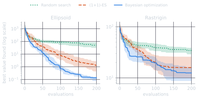
On the smooth ellipsoid, Bayesian optimization was ahead at every budget; comparing every Bayesian run with every evolution strategy run, it found the better point in 80 to 96% of the 900 pairs, depending on the budget. On Rastrigin's function its lead was large at 25 evaluations (83% of pairs) and had nearly vanished by 100 (52%), recovering partly by 200 (64%), and neither method came close to the global minimum. The price was computation: with 199 points observed, one Bayesian proposal took a median 0.092 s on the machine that ran the script, against about 5 microseconds for an evolution strategy step. When an evaluation takes hours, 0.1 s per proposal is negligible and the sample efficiency is decisive; when an evaluation takes microseconds, the evolution strategy can make thousands of evaluations in the time Bayesian optimization makes one proposal, and the cubic cost of the Gaussian process in the number of points makes Bayesian optimization expensive at large budgets in any case.
These are our observations on two toy functions in five dimensions, with a simple evolution strategy rather than CMA-ES; they illustrate the trade-off rather than rank the methods. The no free lunch theorems say that no ranking holds across all problems, and the practical choice depends on what an evaluation costs, how many variables there are, and whether the problem has the structure a model can learn.
References
- Hart, E., Ross, P., and Corne, D. (2005). Evolutionary scheduling: A review. Genetic Programming and Evolvable Machines, 6(2), 191–220.
- Hornby, G. S., Globus, A., Linden, D. S., and Lohn, J. D. (2006). Automated antenna design with evolutionary algorithms. In Proceedings of AIAA Space 2006, AIAA 2006-7242.
- Hornby, G. S., Lohn, J. D., and Linden, D. S. (2011). Computer-automated evolution of an X-band antenna for NASA's Space Technology 5 mission. Evolutionary Computation, 19(1), 1–23.
- Jameson, A. (1988). Aerodynamic design via control theory. Journal of Scientific Computing, 3(3), 233–260.
- Jin, Y. (2011). Surrogate-assisted evolutionary computation: Recent advances and future challenges. Swarm and Evolutionary Computation, 1(2), 61–70.
- Jones, D. R., Schonlau, M., and Welch, W. J. (1998). Efficient global optimization of expensive black-box functions. Journal of Global Optimization, 13(4), 455–492.
- Keane, A. J. (1995). Passive vibration control via unusual geometries: The application of genetic algorithm optimization to structural design. Journal of Sound and Vibration, 185(3), 441–453.
- Keane, A. J. (n.d.). Vibrations in space: Application to satellite truss design. Project poster, Computational Engineering and Design Centre, University of Southampton.
- Keane, A. J., and Bright, A. P. (1996). Passive vibration control via unusual geometries: Experiments on model aerospace structures. Journal of Sound and Vibration, 190(4), 713–719.
- Keane, A. J., and Brown, S. M. (1996). The design of a satellite boom with enhanced vibration performance using genetic algorithm techniques. In Proceedings of Adaptive Computing in Engineering Design and Control '96 (ACEDC '96), Plymouth, UK, 107–113.
- Obayashi, S., Sasaki, D., Takeguchi, Y., and Hirose, N. (2000). Multiobjective evolutionary computation for supersonic wing-shape optimization. IEEE Transactions on Evolutionary Computation, 4(2), 182–187.
- Oyama, A., Liou, M.-S., and Obayashi, S. (2004). Transonic axial-flow blade optimization: Evolutionary algorithms/three-dimensional Navier-Stokes solver. Journal of Propulsion and Power, 20(4), 612–619.
- Paechter, B., Rankin, R. C., Cumming, A., and Fogarty, T. C. (1998). Timetabling the classes of an entire university with an evolutionary algorithm. In Parallel Problem Solving from Nature (PPSN V), Lecture Notes in Computer Science 1498, 865–874. Springer.
- Thompson, A. (1997). An evolved circuit, intrinsic in silicon, entwined with physics. In Evolvable Systems: From Biology to Hardware (ICES 1996), Lecture Notes in Computer Science 1259, 390–405. Springer.
- Times Higher Education (1998). Napier evolves ideal timetable. 13 February 1998.
- Turner, R., Eriksson, D., McCourt, M., Kiili, J., Laaksonen, E., Xu, Z., and Guyon, I. (2021). Bayesian optimization is superior to random search for machine learning hyperparameter tuning: Analysis of the black-box optimization challenge 2020. In Proceedings of the NeurIPS 2020 Competition and Demonstration Track, Proceedings of Machine Learning Research 133, 3–26.