A hill climber with the 2-opt neighborhood, started from a random tour of the 100 cities in the TSPLIB instance kroA100, stops after about a hundred moves at a tour roughly 7% longer than the optimum. Nothing in the neighborhood of that tour is shorter. Every way out goes uphill first, through longer tours, and a hill climber never takes such a step. The methods in this article are different answers to one question: how should a search decide when to accept a worse state, or when to abandon the current state altogether?
There are four broad answers. Start again somewhere else (random restarts). Accept worse moves at random, less and less often over time (simulated annealing). Accept the best available move even when it is worse, and use memory to avoid walking straight back (tabu search). Kick the current local optimum just hard enough to leave its basin, and climb again (iterated local search). A fifth answer, keeping many states at once, leads to evolutionary algorithms. The four single-state methods are compared at the end on kroA100, with every method given the same number of evaluations.
Sideways moves
The cheapest change helps only on plateaus. A hill climber that accepts only strict improvements stops on a shoulder, a flat region with an uphill exit somewhere along its edge. Accepting sideways moves to neighbors of equal value lets it keep walking until it finds the exit. On a flat local maximum, which has no exit, it would walk forever, so the number of consecutive sideways moves must be capped (Russell and Norvig, 2020, §4.1.1).
The 8-queens problem, minimizing the number of pairs of queens that attack each other, shows the size of the effect. In the experiment of hill climbing on 8-queens and the 8-puzzle, 30,000 runs of steepest descent from random placements reached a solution 14.02% of the time. With up to 100 consecutive sideways moves allowed, they reached one 94.28% of the time. The cost was longer climbs, a mean of 19.16 moves for a success and 60.68 for a failure, against 4.09 and 3.05 without sideways moves. The same experiment shows that sideways moves need randomness: when ties between equally good neighbors are broken by a fixed rule, the walk across a plateau falls into a loop, and the success rate with sideways moves is only 32.45%. Sideways moves do nothing for a strict local optimum, where every neighbor is worse, and on most problems with real-valued objectives exact ties are rare. The remaining methods deal with strict local optima.
Random restarts
Random-restart hill climbing runs a hill climber to a local optimum, starts again from a new random state, and keeps the best state found across all climbs. If each climb independently reaches a global optimum with probability $p$, two questions matter: how likely a budget of $k$ climbs is to succeed, and how many climbs are needed on average.
Success within $k$ climbs. The $k$ climbs all fail with probability $(1 - p)^k$, because each fails with probability $1 - p$ independently of the others. At least one succeeds with the complementary probability,
$$P(\text{success within } k \text{ climbs}) = 1 - (1 - p)^k.$$
To succeed with probability at least $c$, set $1 - (1 - p)^k \ge c$, so $(1 - p)^k \le 1 - c$, and take logarithms (both sides of $k \ln(1 - p) \le \ln(1 - c)$ are negative, so dividing by $\ln(1 - p)$ reverses the inequality):
$$k \ge \frac{\ln(1 - c)}{\ln(1 - p)}.$$
Expected number of climbs. The first success comes at climb $k$ when the first $k - 1$ climbs fail and the $k$-th succeeds, with probability $(1 - p)^{k-1} p$. This is the geometric distribution, and its mean is
$$\mathbb{E}[\text{climbs}] = \sum_{k=1}^{\infty} k\,(1 - p)^{k-1} p = \frac{1}{p},$$
using $\sum_{k \ge 1} k q^{k-1} = 1/(1 - q)^2$ with $q = 1 - p$. Of these climbs, on average $1/p - 1 = (1 - p)/p$ fail before the one that succeeds. If a failed climb costs $c_f$ evaluations on average and a successful one $c_s$, the expected cost of finding the optimum is
$$\mathbb{E}[\text{cost}] = c_s + \frac{1 - p}{p}\, c_f.$$
For the 8-queens problem above, $p = 0.1402$, so about 7.1 climbs are needed on average, and the expected number of moves is $4.09 + (0.8598 / 0.1402) \times 3.05 \approx 22.8$. With sideways moves, $p = 0.9428$, and the expected number of moves is $19.16 + (0.0572 / 0.9428) \times 60.68 \approx 22.8$ as well. The two strategies cost about the same; sideways moves buy fewer restarts with longer climbs.
The success formula can be checked directly. The 8-queens experiment ran 10,000 restart trials for each setting, each trial climbing from fresh random boards until one climb succeeded, and recorded how many climbs it took. Without sideways moves:
| Climbs $k$ | Predicted $1 - (1 - 0.1402)^k$ | Measured share of trials solved within $k$ |
|---|---|---|
| 1 | 0.1402 | 0.1385 |
| 2 | 0.2607 | 0.2523 |
| 5 | 0.5301 | 0.5322 |
| 10 | 0.7792 | 0.7753 |
| 20 | 0.9513 | 0.9515 |
| 30 | 0.9892 | 0.9890 |
For 90% confidence the bound asks for $k \ge \ln 0.1 / \ln 0.8598 = 15.2$, so 16 climbs, and 90.90% of the trials finished within 16. For 99%, it asks for 31, and 99.04% finished within 31. With sideways moves, $p = 0.9428$, a single climb succeeds 94.4% of the time in the trials and two climbs 99.7%. The agreement is what independence predicts: each climb starts from a fresh random board and keeps no memory of earlier ones.
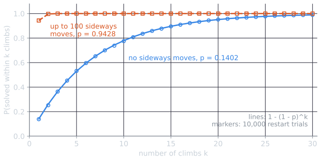
The success probability $p$ is the fraction of the search space inside the basin of attraction of the global optimum, weighted by how starting states are drawn. On small problems it can be computed exactly. The table below uses the NK fitness landscapes of fitness landscapes, with $N = 16$ loci each interacting with $K$ others, the same random instances. Steepest-ascent hill climbing with one-bit flips was run from every one of the $2^{16} = 65{,}536$ starting strings. A climb of $s$ moves costs $1 + 16(s + 1)$ evaluations: the start, one scan per move, and a final scan that finds no improvement. The script is tools/experiments/evolution/hill_climbing.py in the site repository.
| $K$ | Local optima | $p$ | Expected climbs $1/p$ | Mean moves per climb | Expected evaluations to reach the optimum |
|---|---|---|---|---|---|
| 0 | 1 | 1.0000 | 1.0 | 8.0 | 145 |
| 2 | 64 | 0.1266 | 7.9 | 5.0 | 772 |
| 4 | 173 | 0.0352 | 28.4 | 4.1 | 2,337 |
| 8 | 931 | 0.0079 | 127.0 | 2.6 | 7,512 |
| 15 | 3,813 | 0.0007 | 1,337.5 | 1.6 | 56,182 |
As epistasis grows, the basin of the global optimum shrinks, the climbs get shorter, and the number of restarts needed grows quickly. On these small instances restarts are still effective. With $K = 4$, random restarts need about 2,300 evaluations on average, while the $(1+1)$ EA in fitness landscapes found the optimum of the same instance in only 10 of 30 runs within 20,000 evaluations.
Restarts become less useful as problems grow. Each climb is an independent sample from the distribution of local optima, so restarts can only find what that distribution puts some weight on. Lourenço, Martin, and Stützle (2003) point out that on large instances, empirical studies and general arguments indicate that the costs of local optima found from random starts have a mean a fixed percentage above the optimum and a distribution that becomes more and more sharply peaked around that mean as the instance grows. Independent sampling then almost never reaches the lower tail, where the good solutions are. The remaining methods search near good solutions already found instead of sampling afresh.
Simulated annealing
Simulated annealing accepts worse moves at random, with a probability that depends on how much worse they are and on a parameter, the temperature, that falls during the run. It comes from statistical physics. To estimate the properties of a system of interacting particles, Metropolis, Rosenbluth, Rosenbluth, Teller, and Teller (1953) moved one particle at a time and accepted a move that changed the energy by $\Delta$ always if $\Delta \le 0$, and otherwise with probability $e^{-\Delta / kT}$. Run long enough at a fixed temperature, this process samples states with the Boltzmann distribution, in which a state of energy $E$ has probability proportional to $e^{-E/kT}$. At low temperature that distribution is concentrated on the lowest-energy states. Kirkpatrick, Gelatt, and Vecchi (1983) proposed treating the cost of an optimization problem as the energy, and lowering the temperature slowly, as a metal is annealed by slow cooling to reach a low-energy crystal structure. They applied the method to the partitioning and placement of circuits on computer chips and to the travelling salesman problem. Černý (1985) developed the same idea independently for the travelling salesman problem.
For minimizing a cost $f$, with the constant $k$ absorbed into $T$:
- Start from a state $x$ and a temperature $T_0$.
- At step $k$, draw a neighbor $y$ of $x$ uniformly at random and compute $\Delta = f(y) - f(x)$.
- If $\Delta \le 0$, move to $y$. Otherwise move to $y$ with probability $e^{-\Delta / T_k}$.
- Lower the temperature according to the cooling schedule, and repeat until the budget runs out. Keep the best state seen.
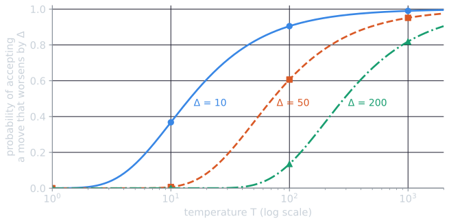
At high temperature nearly every move is accepted, and the search is close to a random walk. At low temperature almost no worsening move is accepted, and the search is a first-choice hill climber. The schedule controls the passage between the two. For a move that lengthens a tour by 50, the acceptance probability is $e^{-0.5} = 0.61$ at $T = 100$, $e^{-5} = 0.0067$ at $T = 10$, and $e^{-50} \approx 2 \times 10^{-22}$ at $T = 1$. The same calculation for three sizes of worsening move, rounded to three significant figures:
| Increase $\Delta$ | $T = 1$ | $T = 10$ | $T = 100$ | $T = 1000$ |
|---|---|---|---|---|
| 10 | $4.54 \times 10^{-5}$ | 0.368 | 0.905 | 0.990 |
| 50 | $1.93 \times 10^{-22}$ | 0.00674 | 0.607 | 0.951 |
| 200 | $1.38 \times 10^{-87}$ | $2.06 \times 10^{-9}$ | 0.135 | 0.819 |
Two things are visible. The temperature has the same units as the cost, and what matters is the ratio $\Delta / T$: a move is accepted about half the time when $\Delta \approx 0.69\,T$, since $e^{-0.69} \approx 0.5$. And at every temperature, small worsening moves are accepted far more readily than large ones, so annealing climbs out of shallow valleys long before it climbs out of deep ones.
What annealing does at a fixed temperature
Before cooling enters, it helps to see what the acceptance rule achieves when $T$ is held fixed. Take the one-dimensional example of hill climbing, with states $x = 0, \ldots, 60$, neighbors $x \pm 1$, and integer heights $f(x)$ from 3 to 21 to be maximized, with the global maximum $f(36) = 21$. Annealing proposes $x - 1$ or $x + 1$ with probability $\tfrac{1}{2}$ each (a proposal off either end is refused), accepts a rise always, and accepts a fall of $d$ with probability $e^{-d/T}$.
Run long enough at fixed $T$, this process spends a fraction of its time at each state given by the Boltzmann distribution
$$\pi_T(x) = \frac{e^{f(x)/T}}{\sum_{z} e^{f(z)/T}},$$
the maximization version of the $e^{-E/kT}$ of Metropolis and colleagues. The reason is a balance between neighboring states. Let $y$ be a neighbor of $x$ with $f(y) < f(x)$. The probability of being at $x$ and moving to $y$ in one step is $\pi_T(x) \cdot \tfrac{1}{2} \cdot e^{-(f(x) - f(y))/T}$. The probability of being at $y$ and moving to $x$ is $\pi_T(y) \cdot \tfrac{1}{2} \cdot 1$, since a rise is always accepted. Substituting $\pi_T$, both equal $\tfrac{1}{2} e^{f(y)/T} / \sum_z e^{f(z)/T}$. When the flow in each direction between every pair of neighbors is equal (the detailed balance condition), the total flow into each state equals the flow out, so $\pi_T$ does not change from one step to the next: it is the chain's stationary distribution. Because the chain can reach every state and can stay put (at the ends, and whenever a fall is refused), it converges to $\pi_T$ from any start.
The Boltzmann distribution makes the role of the temperature exact. The higher a state, the more weight it gets, and lowering $T$ sharpens the preference:
| Temperature | $\pi_T(36)$ | $\pi_T(35) + \pi_T(36) + \pi_T(37)$ | Flat maximum, $x = 45$ to 50 | Local maximum, $x = 8$ |
|---|---|---|---|---|
| 5 | 0.0579 | 0.1527 | 0.1907 | 0.0078 |
| 2 | 0.1630 | 0.3607 | 0.2182 | 0.0011 |
| 1 | 0.3959 | 0.6872 | 0.1183 | $1.8 \times 10^{-5}$ |
| 0.5 | 0.7526 | 0.9563 | 0.0112 | $1.6 \times 10^{-9}$ |
At $T = 5$ the flat maximum, six states at height 18, holds more probability than the single global maximum; at $T = 0.5$ three quarters of the time is spent at $x = 36$. As $T \to 0$ the distribution concentrates entirely on the global maxima. That is the idea of annealing in one sentence: sample the Boltzmann distribution, and lower the temperature so that it concentrates on the best states. The catch is time. At low temperature the chain needs a very long time to reach its stationary distribution, because leaving the local maximum at $x = 8$ requires six consecutive downhill steps, each accepted with probability $e^{-1/T}$ and proposed with probability $\tfrac{1}{2}$, about $(e^{-1/T}/2)^6$ in all, which is $7.8 \times 10^{-4}$ at $T = 2$ and $9.6 \times 10^{-8}$ at $T = 0.5$. A schedule has to keep the temperature high long enough for the search to move between basins, and lower it slowly enough that it settles in the right one.
Cooling schedules
The most common schedule in practice is geometric: $T_{k+1} = \alpha T_k$ for a constant $\alpha$ slightly below 1. The experiment below cools geometrically from $T_0 = 100$ to $T = 1$ over the whole run, which for 2 million steps means $\alpha = 0.01^{1/2{,}000{,}000} \approx 0.9999977$.
The figure below follows one of those runs (seed 0 of the experiment later in this article) through its 2 million steps. It found a tour of length 21,431, 0.70% above the optimum.
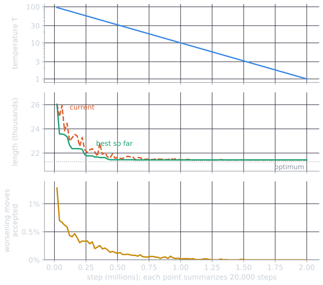
Three features of this run are worth reading off the plot. First, even at the start, with $T$ close to 100, only 1.28% of the proposed worsening moves were accepted. The reason is the size of a typical move: a 2-opt move chosen at random usually joins cities that are far apart, and the median increase among the worsening moves proposed in each window was between 2,570 and 2,849. At $T = 100$ an increase of 2,570 is accepted with probability $e^{-25.7} \approx 7 \times 10^{-12}$, so the worsening moves that were accepted were the rare small ones: 2,184 of them over the run, with a median increase of 49, nine in ten below 180, and none above 563. Second, the best tour of the run was found at step 635,286, when $T$ was about 23; the current tour kept moving above it and was back at the same length by about 1.2 million steps. The last accepted worsening move came at step 1,490,922, and after step 1,496,923 the tour never changed again, so the final quarter of the budget was spent proposing moves that were all refused. Third, the useful range of temperatures is set by the sizes of the moves that matter, increases of tens to a few hundreds here, not by the typical proposed move. The temperatures used, from 100 to 1, were chosen in a small pilot, described below. This run shows that they work, and it suggests that for this instance the lowest temperatures add little.
Whether annealing finds a global optimum with certainty, given enough time, was settled for finite problems in the 1980s. Geman and Geman (1984), working on image restoration with a related sampler, proved convergence to the global minima for schedules of the form
$$T_k = \frac{c}{\log(k + 1)}$$
when the constant $c$ is large enough (log is the natural logarithm). Hajek (1988) found the exact condition. Assume that the state space is finite, that any state can be reached from any other by a sequence of moves, and that the neighborhood satisfies weak reversibility: if state $j$ can be reached from state $i$ without passing through any state of cost above $E$, then $i$ can be reached from $j$ in the same way. (A symmetric neighborhood, such as 2-opt, satisfies this.) The depth of a local minimum $s$ that is not global is the smallest $d > 0$ such that some state of lower cost than $s$ can be reached from $s$ without exceeding cost $f(s) + d$: the height of the lowest pass out of its valley. Let $d^*$ be the largest depth of any local minimum that is not global, and suppose $T_k$ is nonincreasing and tends to 0. Hajek's theorem states that the probability that the state at step $k$ is a global minimum tends to 1 if and only if
$$\sum_{k=1}^{\infty} e^{-d^* / T_k} = \infty.$$
For the logarithmic schedule, $e^{-d^* \log(k+1)/c} = (k+1)^{-d^*/c}$, and this series diverges exactly when $d^*/c \le 1$. Annealing with $T_k = c/\log(k+1)$ therefore converges if and only if $c \ge d^*$.
The theorem guarantees convergence, not speed, and the logarithmic schedule is extremely slow. With $T_k = c / \log(k + 1)$, the temperature falls to a tenth of $c$ only after about 22,000 steps, to a twentieth after about $4.9 \times 10^8$, and lowering it from 100 at the first step to 1 would take about $2^{100} \approx 1.3 \times 10^{30}$ steps. Practical schedules cool much faster and give up the guarantee. Simulated annealing as used is a heuristic whose schedule must be tuned, with convergence theory as a statement about the limit.
Hajek's condition on a small example
The one-dimensional example is small enough to apply the theorem by hand and then to compute exactly what happens. The theorem is stated for minimizing a cost; for maximizing $f$, the depth of a local maximum is how far the search must go down before it can reach a strictly higher state. It has three local maxima that are not global:
- $x = 8$, height 11. Every higher state lies to the right, and the path there passes through the valley at $x = 14$, height 5. Its depth is $11 - 5 = 6$.
- the flat maximum $x = 45$ to 50, height 18. To its left, the path to the global maximum passes through $x = 42$, height 15: depth 3. (To its right nothing is higher.)
- $x = 60$, height 16. The nearest higher states are on the flat maximum, through the valley at $x = 56$, height 12: depth 4.
The shoulder is not a local maximum in this sense, since a higher state can be reached from it without going down at all. So $d^* = 6$, and the theorem says that annealing with $T_k = c / \log(k + 1)$ converges to the global maximum with probability tending to 1 if and only if $c \ge 6$.
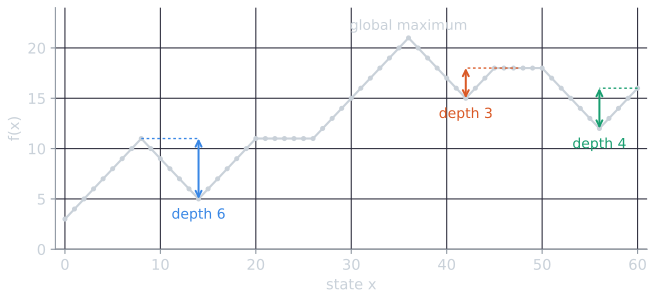
An informal argument, not Hajek's proof, shows why the condition has this form. Take the peak at $x = 8$. To leave it, the search must accept falls totalling 6, which at temperature $T_k$ has probability of order $e^{-6/T_k}$. With $T_k = c/\log(k + 1)$ that is $(k + 1)^{-6/c}$. For $c = 6$ it is $1/(k + 1)$, and the sum of these chances over all steps diverges, like the harmonic series, so a search caught there gets unboundedly many opportunities to leave. For $c = 2$ it is $(k + 1)^{-3}$, whose sum is finite, so with positive probability the search never leaves at all. Hajek's proof makes this precise by estimating how long the chain takes to leave the neighborhood of each local minimum, and the deepest trap is the one that sets the constant.
The chain is also small enough that its distribution can be computed exactly, step by step, with no sampling: start with probability $1/61$ on each state and apply the transition probabilities of the annealing step a million times. Four schedules were compared. Two are logarithmic, with $c = 6 = d^*$ and $c = 2 < d^*$. One is geometric, cooling from 10 to 0.1 over the million steps. One holds $T = 0.5$ fixed. The probability of being at the global maximum $x = 36$, rounded to four decimals:
| Schedule | $k = 10^2$ | $k = 10^3$ | $k = 10^4$ | $k = 10^5$ | $k = 10^6$ |
|---|---|---|---|---|---|
| Logarithmic, $c = 6$ | 0.1389 | 0.3239 | 0.5183 | 0.6519 | 0.7536 |
| Logarithmic, $c = 2$ | 0.3365 | 0.4345 | 0.4541 | 0.4604 | 0.4625 |
| Geometric, 10 to 0.1 | 0.0265 | 0.0329 | 0.0346 | 0.0470 | 0.9953 |
| Fixed, $T = 0.5$ | 0.3158 | 0.3634 | 0.4576 | 0.5905 | 0.6875 |
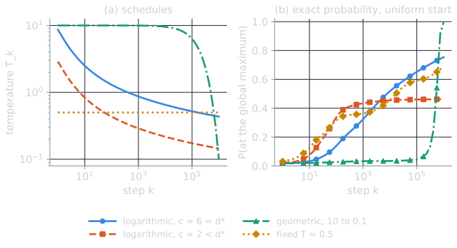
The table shows the theorem and its limits at once. With $c = 2$, cooling is too fast for the deepest trap: the probability of being at the global maximum climbs early and then stops near 0.46, and the probability of being at $x = 8$ stays near 0.24 (0.2372 at a million steps), which is the mass that never escaped. With $c = 6$, the probability at $x = 8$ falls (0.0606 at a million steps) and the probability at the global maximum keeps rising, as the theorem promises, but at a million steps it is still only 0.75. Holding $T = 0.5$ fixed cannot do better than the Boltzmann value 0.7526 in the limit, and the chain is still approaching it. The geometric schedule, which carries no guarantee, ends at 0.9953, the best of the four by a wide margin, because it spends most of the run hot enough to move freely between basins and then cools steadily through the range where the global maximum takes over. A schedule that is provably convergent in the limit can lose badly at a fixed budget, which is why practice uses fast schedules tuned to the problem. The exact computation, like the other worked examples in this article (the acceptance table, the annealing run, the tabu trace and the restart check), is in tools/experiments/evolution/escaping_examples.py in the site repository.
Tabu search
Tabu search, introduced by Glover (1986) and developed systematically in Glover (1989, 1990), takes a deterministic route. At every step it moves to the best neighbor, even if that neighbor is worse than the current state. On its own this would cycle: from a local optimum, the best move goes slightly uphill, and the best move from there goes straight back down. Tabu search prevents this with short-term memory. Some attribute of each recent move, such as the edges a 2-opt move removed, is declared tabu for a fixed number of iterations, the tabu tenure, and moves that would restore a tabu attribute are forbidden. An aspiration criterion overrides the prohibition for a move good enough to be worth making anyway, most simply one that would produce the best state found so far.
The version used below for the TSP is:
- Start from a random tour. At each iteration, evaluate every 2-opt move.
- A move is tabu if either edge it would add was removed within the last 40 iterations. A tabu move is still admissible if it would produce a tour shorter than the best found so far.
- Make the admissible move with the smallest change in length, whether that change is negative or positive (ties broken by move order), and mark the two removed edges tabu for 40 iterations. If no move is admissible, the iteration makes no move.
- Keep the best tour found, and stop when the budget is spent.
Because it evaluates the whole neighborhood every iteration, tabu search pays the cost of steepest ascent at every step. The tenure governs the balance between staying near good solutions and moving away. Too short, and the search falls back into the local optimum it just left; too long, and good moves stay forbidden. Glover's full method adds longer-term memory for intensification and diversification, which the plain version here omits.
A trace on twelve cities
The mechanism is easiest to follow on an instance small enough to solve exactly. Take the first 12 cities of kroA100, numbered 0 to 11, with 54 possible 2-opt moves per tour. The Held-Karp dynamic program gives the optimal tour length, 9,775. Steepest descent from a seeded random tour (length 21,857) stops at a 2-opt local optimum of length 9,842, 0.7% too long, and tabu search starts from there with tenure 3: an edge removed at iteration $i$ cannot be added back at iterations $i + 1$ and $i + 2$, unless the aspiration criterion applies.
Without memory (tenure 0), the search cycles at once. The best move from the local optimum lengthens the tour by 11, by removing the edges 2-11 and 8-10 and adding 2-8 and 11-10. From the new tour the best move is its exact reverse, which shortens the tour by 11, and the search alternates between the two tours forever.
With tenure 3, the reverse move is forbidden, and the search is pushed further:
| Iteration | Edges removed | Edges added | Change | Length | Best | Better moves that were tabu |
|---|---|---|---|---|---|---|
| 1 | 2-11, 8-10 | 2-8, 11-10 | +11 | 9,853 | 9,842 | none |
| 2 | 2-8, 6-11 | 2-6, 8-11 | +32 | 9,885 | 9,842 | -11 (adds 2-11, 8-10) |
| 3 | 9-3, 5-0 | 9-5, 3-0 | +113 | 9,998 | 9,842 | -32 (adds 2-8, 6-11); -1 (adds 2-11) |
| 4 | 3-0, 7-1 | 3-7, 0-1 | -180 | 9,818 | 9,818 | none |
| 5 | 2-6, 8-11 | 2-8, 6-11 | -32 | 9,786 | 9,786 | none |
| 6 | 2-8, 11-10 | 2-11, 8-10 | -11 | 9,775 | 9,775 | none |
In iteration 2 the best move by far would undo iteration 1, and it is tabu because it adds back two edges removed one iteration earlier. In iteration 3 two better moves are tabu, and the search accepts a large increase of 113. That increase is what opens the way: the move in iteration 4 shortens the tour by 180, leaving it shorter than the starting local optimum, and two more improving moves reach the optimum at iteration 6. Iterations 5 and 6 add back edges removed in iterations 2 and 1, which is allowed because their tenure has expired. The whole escape took three uphill moves totalling +156 followed by three downhill moves totalling -223.
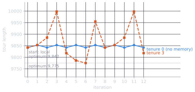
The trace also shows the limit of short-term memory. After reaching the optimum, the search has to keep moving, so it takes the least bad move that is not tabu (+180; two smaller increases, +11 and +42, are tabu), which undoes iteration 4. Iteration 8 undoes iteration 3 and returns to the starting tour, and from iteration 9 the whole sequence repeats with period 8. A tenure of 3 forbids only moves that undo the last two iterations, so it cannot prevent a longer cycle. In practice the tenure is set long enough to make cycles rare, the experiment below uses 40 on 100 cities, and the best tour found is kept regardless of where the search wanders afterwards.
Iterated local search
Iterated local search treats a hill climber as a black box and searches the space of its local optima (Lourenço, Martin, and Stützle, 2003). Its structure is:
- Run the local search from an initial state to a local optimum $s^*$.
- Perturb $s^*$ to get a new state $s'$.
- Run the local search from $s'$ to a local optimum $s^{*\prime}$.
- Apply an acceptance criterion to choose between $s^*$ and $s^{*\prime}$ as the new current state, and return to step 2.
The perturbation must be strong enough that the local search does not simply return to $s^*$, and weak enough that the result is not effectively a random restart. For the TSP, the standard perturbation is the double-bridge move: cut the tour into four segments $A\,B\,C\,D$ and reconnect them as $A\,C\,B\,D$. Lourenço, Martin, and Stützle (2003) note that nearly all iterated local search studies of the TSP use this kind of perturbation, which changes four edges, can join cities that are far apart, and is not easily undone by 2-opt, 3-opt, or Lin-Kernighan local search. It descends from the large-step Markov chains of Martin, Otto, and Felten (1991), which applied a special four-edge change followed by local search, with an annealing-like acceptance rule. The acceptance criterion ranges from Better, which accepts $s^{*\prime}$ only if it improves on $s^*$, to a random walk that always accepts it. The version used below accepts $s^{*\prime}$ if it is no longer than $s^*$, uses steepest-descent 2-opt as the local search, and chooses the three cut points uniformly at random.
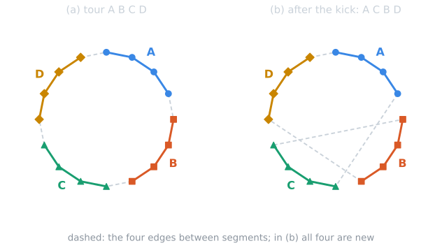
Why this particular kick? It keeps all four segments in their original direction and swaps the middle two, a change of four edges, which no single 2-opt or 3-opt move (changing two or three edges) can make or undo. And after the kick, most of the tour is still as good as before: only the four new edges, which may join distant cities, are likely to be poor, and the local search has to repair the tour only around them. That is why the descent after a kick is short, as the experiment below measures.
The four methods side by side
| Method | How it leaves a local optimum | What it remembers | Settings that decide its behavior |
|---|---|---|---|
| Random restarts | abandons it and starts from a new random state | the best state found | none beyond the climber |
| Simulated annealing | accepts a worse neighbor with probability $e^{-\Delta/T}$ | nothing | starting temperature, cooling schedule |
| Tabu search | always takes the best allowed neighbor, worse or not | recently changed attributes | tenure, aspiration rule |
| Iterated local search | kicks it and climbs again, keeping the result if acceptable | the current local optimum | kick strength, acceptance rule |
Experiment: four methods at equal budgets
The four methods were compared on kroA100 (100 cities, optimal tour length 21,282), all with the 2-opt neighborhood. An evaluation is the computation of one move's change in tour length, and every run of every method had the same budget of evaluations, starting from a random tour.
- Hill climbing with restarts: steepest-descent 2-opt to a local optimum, then a new random tour, until the budget is spent.
- Simulated annealing: one random 2-opt move per evaluation, geometric cooling from $T_0 = 100$ to $T = 1$ over the budget.
- Tabu search: as specified above, with tenure 40 (an edge removed at one iteration stays tabu through the next 39).
- Iterated local search: as specified above.
The annealing temperatures and the tabu tenure were chosen in a small pilot on seeds outside the reported runs, at the smaller budget, and were not retuned for the larger one. Each method had 30 seeded runs. The table gives the median excess of the best tour over the optimum, with the interquartile range, and the number of runs that found an optimal tour.
| Method | 2 million evaluations | Optimal | 10 million evaluations | Optimal |
|---|---|---|---|---|
| Hill climbing with restarts | 4.64% (3.33 to 5.12) | 0 / 30 | 1.93% (1.33 to 2.61) | 0 / 30 |
| Simulated annealing | 0.49% (0.30 to 0.84) | 4 / 30 | 0.44% (0.26 to 0.62) | 3 / 30 |
| Tabu search | 3.20% (2.21 to 4.29) | 0 / 30 | 1.79% (0.93 to 2.73) | 0 / 30 |
| Iterated local search | 2.27% (1.35 to 3.02) | 0 / 30 | 0.40% (0.01 to 1.10) | 8 / 30 |
At 2 million evaluations, simulated annealing is far ahead, and the reason is the cost of a step. Annealing spends one evaluation per move. The other three scan all 4,850 moves before each move, so 2 million evaluations allow them only 412 full scans. A steepest descent from a random tour needs about 100 of those, which left hill climbing with restarts a median of 3 complete climbs, and tabu search 412 iterations in total, a quarter of them spent on the first descent. Iterated local search did better than both because after a double-bridge kick only a few edges are wrong, and the descent back to a local optimum takes a few scans instead of a hundred; it completed a median of 59 kicks.
At 10 million evaluations, the order changes. Hill climbing with restarts improves, with 19 climbs per run, but remains the weakest. Tabu search, with 2,061 iterations, improves to about the same level. Iterated local search, with a median of 384 kicks, now matches simulated annealing in median and found the optimum in 8 runs, although its spread is wider. Simulated annealing barely improves with the longer schedule. Its temperatures were tuned at the smaller budget, and a schedule that cools five times more slowly is not automatically better.
These numbers describe plain textbook implementations on one instance, and they should not be read as a general ranking. Fast implementations restrict each scan to candidate lists of each city's nearest neighbors and, in iterated local search, skip cities whose surroundings have not changed since the last scan (Lourenço, Martin, and Stützle, 2003). That greatly reduces the cost of a step, increasingly so on larger instances, and would change this comparison. The general point survives that caveat. Comparisons at an equal budget depend on what a step costs, and every method here has parameters, such as a schedule, a tenure, or a perturbation strength, that decide its behavior as much as its idea does. The No Free Lunch theorems add that no ranking can hold over all problems. The script is tools/experiments/evolution/local_search.py in the site repository.
A population as another answer
Every method above follows a single trajectory, and escapes by changing how that trajectory moves. A different answer is to keep many states at once. Russell and Norvig (2020, §4.1.3) describe local beam search, which keeps $k$ states, generates all their neighbors, and keeps the best $k$ of the combined set. It is not the same as $k$ independent restarts: states with good neighbors attract the search, and the beam can collapse onto one region. Their stochastic beam search chooses the $k$ survivors at random with probability increasing in fitness, which, as Russell and Norvig observe (2020, §4.1.3–4.1.4), resembles natural selection and leads directly to evolutionary algorithms.
An evolutionary algorithm adds two things to a stochastic beam. Recombination builds new states from parts of several existing ones, so a population can combine features that separate trajectories found independently. Selection pressure, how strongly the fitter states are preferred, then plays a part similar to temperature in annealing: strong pressure behaves like hill climbing and loses diversity quickly (selection pressure and premature convergence), and weak pressure behaves like a random walk. The simple genetic algorithm is the standard example. Population methods and local search are also combined: Eiben and Smith (2015, ch. 10) describe memetic algorithms, which apply local search to the members of an evolving population, so that the population explores and the local search refines.
References
- Černý, V. (1985). Thermodynamical approach to the traveling salesman problem: An efficient simulation algorithm. Journal of Optimization Theory and Applications, 45(1), 41–51.
- Eiben, A. E., and Smith, J. E. (2015). Introduction to Evolutionary Computing, 2nd ed., chapter 10. Springer.
- Geman, S., and Geman, D. (1984). Stochastic relaxation, Gibbs distributions, and the Bayesian restoration of images. IEEE Transactions on Pattern Analysis and Machine Intelligence, PAMI-6(6), 721–741.
- Glover, F. (1986). Future paths for integer programming and links to artificial intelligence. Computers & Operations Research, 13(5), 533–549.
- Glover, F. (1989). Tabu search, part I. ORSA Journal on Computing, 1(3), 190–206.
- Glover, F. (1990). Tabu search, part II. ORSA Journal on Computing, 2(1), 4–32.
- Hajek, B. (1988). Cooling schedules for optimal annealing. Mathematics of Operations Research, 13(2), 311–329.
- Kirkpatrick, S., Gelatt, C. D., Jr., and Vecchi, M. P. (1983). Optimization by simulated annealing. Science, 220(4598), 671–680.
- Lourenço, H. R., Martin, O. C., and Stützle, T. (2003). Iterated local search. In F. Glover and G. A. Kochenberger (Eds.), Handbook of Metaheuristics, 320–353. Kluwer Academic Publishers.
- Martin, O., Otto, S. W., and Felten, E. W. (1991). Large-step Markov chains for the traveling salesman problem. Complex Systems, 5(3), 299–326.
- Metropolis, N., Rosenbluth, A. W., Rosenbluth, M. N., Teller, A. H., and Teller, E. (1953). Equation of state calculations by fast computing machines. Journal of Chemical Physics, 21(6), 1087–1092.
- Russell, S., and Norvig, P. (2020). Artificial Intelligence: A Modern Approach, 4th ed., section 4.1. Pearson.