Take the expression $((x + 1) \cdot x) + 1$, which equals $x^2 + x + 1$, the target of the classic symbolic regression example. As a program tree it has three internal nodes and four leaves, and tree-based genetic programming (GP) evolves it by swapping and regrowing subtrees. The same expression can also be written as register instructions, as integers wiring up a small graph, as bytes read through a grammar, or as a postfix program for a stack machine. Each of these has become a full GP system, and each changes what a mutation does and which parts of the genome are expressed.
The course, like the textbook, presents GP with trees (Eiben and Smith, 2015, ch. 6). This article decodes a genotype of each of four other representations by hand into the expression above, then turns to the claims of human-competitive results for GP and to program search with large language models. The decodings and counts quoted below are printed by tools/experiments/evolution/gp_representations.py in the site repository.
Genotype and phenotype in GP
In tree GP the genotype is the program: variation operators act directly on the parse tree that is executed. Miller and Thomson (2000) pointed out that this leaves no room for a genotype-phenotype mapping, the distinction that the general evolutionary algorithm draws between an encoding and the solution it describes. All four representations below introduce one. A mapping can speed up execution, let parts of a program be reused, guarantee syntactically valid offspring, or let many genotypes map to the same phenotype. That last property, redundancy, creates neutral mutations, which leave fitness unchanged (see fitness landscapes). The cost is that a small change to the genotype need not be a small change to the program, a problem familiar from binary encoding.
Linear GP
Linear genetic programming represents a program as a sequence of instructions for a register machine, in the style of an imperative language or of machine code (Brameier and Banzhaf, 2007). The typical instruction has three addresses, $r_i := r_j \;\mathit{op}\; r_k$: it reads two registers, or a register and a constant, applies an operator, and writes the result to a destination register. Some registers hold the program inputs before execution, additional calculation registers are initialized to a fixed value, such as 1, before each run on a fitness case, constants live in write-protected registers, and one register is designated the output (Brameier and Banzhaf, 2007, ch. 2).
Worked example
Let register $r_0$ hold the input $x$ and serve as the output, let $r_1, r_2, r_3$ be calculation registers set to 1, and let "1" denote a constant. The program has seven instructions. The trace shows the registers after each one, for $x = 2$:
| # | Instruction | $r_0, r_1, r_2, r_3$ at $x = 2$ | Status |
|---|---|---|---|
| 1 | $r_1 := r_0 + 1$ | 2, 3, 1, 1 | effective |
| 2 | $r_3 := r_0 \cdot r_0$ | 2, 3, 1, 4 | structural intron |
| 3 | $r_2 := r_1 \cdot r_0$ | 2, 3, 6, 4 | effective |
| 4 | $r_3 := r_2 - r_1$ | 2, 3, 6, 3 | structural intron |
| 5 | $r_2 := r_2 \cdot 1$ | 2, 3, 6, 3 | effective (a semantic intron) |
| 6 | $r_0 := r_2 + 1$ | 7, 3, 6, 3 | effective |
| 7 | $r_3 := r_3 \cdot r_3$ | 7, 3, 6, 9 | structural intron |
The output is $r_0 = 7 = 2^2 + 2 + 1$. Instructions 2, 4 and 7 write to $r_3$, which nothing on the path to the output ever reads, so they cannot affect the result for any input.
Effective and non-effective code
Brameier and Banzhaf (2007, ch. 3) call an instruction effective if it can influence the program output for some input, and distinguish two kinds of non-effective code, or introns. A structural intron writes to a register that is not effective at that point in the program: no later instruction on the path to the output reads its result. A semantic intron writes to an effective register but leaves its value unchanged, as $r_2 := r_2 \cdot 1$ does here. Structural introns arise from the imperative form itself and have no counterpart in tree GP, where every node is connected to the root.
Structural introns can be found exactly with one backward pass. Start with the set of effective registers $\{r_0\}$ and walk backward. An instruction whose destination is in the set is effective; its destination leaves the set and its operand registers join it. An instruction whose destination is not in the set is an intron and leaves the set unchanged:
| Instruction | Destination | Effective set before | Decision | Effective set after |
|---|---|---|---|---|
| 7: $r_3 := r_3 \cdot r_3$ | $r_3$ | $\{r_0\}$ | intron | $\{r_0\}$ |
| 6: $r_0 := r_2 + 1$ | $r_0$ | $\{r_0\}$ | effective | $\{r_2\}$ |
| 5: $r_2 := r_2 \cdot 1$ | $r_2$ | $\{r_2\}$ | effective | $\{r_2\}$ |
| 4: $r_3 := r_2 - r_1$ | $r_3$ | $\{r_2\}$ | intron | $\{r_2\}$ |
| 3: $r_2 := r_1 \cdot r_0$ | $r_2$ | $\{r_2\}$ | effective | $\{r_0, r_1\}$ |
| 2: $r_3 := r_0 \cdot r_0$ | $r_3$ | $\{r_0, r_1\}$ | intron | $\{r_0, r_1\}$ |
| 1: $r_1 := r_0 + 1$ | $r_1$ | $\{r_0, r_1\}$ | effective | $\{r_0\}$ |
The set left at the end, $\{r_0\}$, lists the registers whose initial values the program uses: only the input. Instruction 4 is the instructive case. It reads $r_2$ and $r_1$, both of which carry effective values at that point, but it writes $r_3$, and the only later reader of $r_3$ is instruction 7, itself an intron. Reading useful values does not make an instruction useful; what matters is whether its result reaches the output. Semantic introns cannot be found this way, because detecting them depends on what the operations compute.
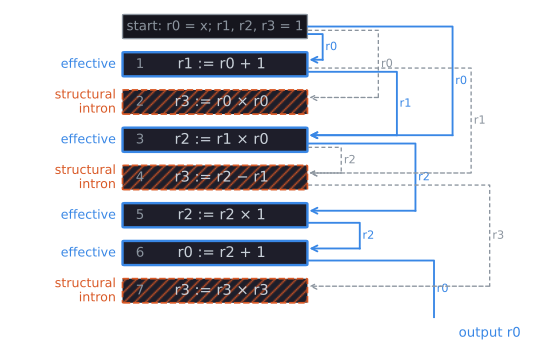
Two consequences follow. First, the evaluator can remove the structural introns from a copy of the program and execute only the effective code, while the full genotype, introns included, stays in the population (Brameier and Banzhaf, 2007, ch. 3). The script confirms that the four effective instructions, and the three left after also deleting the semantic intron, compute the same values as the full program. Second, a mutation that changes only the operator or operands of a structural intron is neutral. The functional structure of a linear program is also not restricted to a tree: in the example, $r_0$ is read by both instruction 1 and instruction 3, so one stored value feeds two later computations, and the data flow forms a directed acyclic graph (Brameier and Banzhaf, 2007, ch. 3).
Cartesian GP
Cartesian genetic programming (CGP), introduced by Miller and Thomson (2000) after Miller's work on evolving Boolean functions with the same kind of encoding, makes the graph explicit. Nodes sit on a grid of $n_r$ rows and $n_c$ columns. Each node has a function and connections to program inputs or to nodes in earlier columns, which keeps the graph acyclic, and the levels-back parameter $l$ limits how many columns back a connection may reach. The genotype is a fixed-length list of integers. With $n_n$ connections per node and $n_o$ program outputs, its length is $n_r n_c (n_n + 1) + n_o$, but the program it encodes can have any size from zero nodes up to the whole grid (Miller and Thomson, 2000). Miller and Thomson note that the most freely connected form is a single row with $l = n_c$, in which any node can take input from any node to its left. Miller (2011) describes this original form of CGP in full.
Worked example
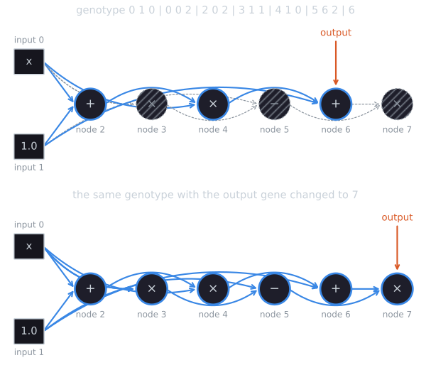
Use one row of six nodes with $l = 6$, two connections per node, and functions numbered 0 for $+$, 1 for $-$ and 2 for $\times$. The inputs are numbered 0 for $x$ and 1 for the constant 1.0, the same pair of inputs Miller and Thomson (2000) used for symbolic regression, and the nodes are numbered 2 to 7. Each node is written as two connection genes followed by a function gene, and one output gene comes last, for $1 \cdot 6 \cdot 3 + 1 = 19$ genes:
0 1 0 | 0 0 2 | 2 0 2 | 3 1 1 | 4 1 0 | 5 6 2 | 6
| Node | Genes | Computes | Value at $x = 2$ | Status |
|---|---|---|---|---|
| 2 | 0 1 0 | $x + 1$ | 3 | active |
| 3 | 0 0 2 | $x \cdot x$ | 4 | inactive |
| 4 | 2 0 2 | node 2 $\cdot\, x$ | 6 | active |
| 5 | 3 1 1 | node 3 $- 1$ | 3 | inactive |
| 6 | 4 1 0 | node 4 $+ 1$ | 7 | active |
| 7 | 5 6 2 | node 5 $\cdot$ node 6 | 21 | inactive |
Decoding traces back from the output gene: node 6 reads node 4 and input 1, node 4 reads node 2 and input 0, and node 2 reads both inputs. The active nodes 2, 4 and 6 spell $((x + 1) \cdot x) + 1$. The output does not depend on nodes 3, 5 and 7, and their nine genes are not expressed.
Neutrality
Every gene has a fixed set of valid values: a function gene takes one of three, a connection gene of the node numbered $k$ takes any of $0, \dots, k - 1$, and the output gene any of $0, \dots, 7$. Changing one gene to each of its other valid values gives 61 single-gene mutants of this genotype. The script finds that 30 of them leave the active graph, and so the program, unchanged: exactly the 30 that alter a gene of an inactive node. None of the other 31 happens to compute the same function on the test points. In the other direction, changing the output gene from 6 to 7 activates every node at once, and the program becomes $(x^2 - 1)\,((x + 1)\,x + 1)$. One point mutation can make a large change, and inactive genes that drifted while unexpressed can suddenly matter.
This is the property CGP is designed to exploit. Most CGP implementations use only point mutation, inside a variant of the $(1+4)$ evolution strategy in which an offspring replaces the parent whenever it is at least as fit, so the search can drift through genotypes of equal fitness (Miller and Harding, 2008). Miller and Thomson (2000) compared that kind of neutral search with a variant that accepted only strictly better genotypes on the Santa Fe ant trail problem and found the neutral search much more effective. In the script's random genotypes of ten nodes with the same function set, over 30 seeds, the median proportion of active nodes is 0.30 (interquartile range 0.20 to 0.40), and the median proportion of single-gene mutations that leave the active graph unchanged is 0.73 (0.65 to 0.84).
Grammatical evolution
Grammatical evolution (GE) (Ryan, Collins, and O'Neill, 1998; O'Neill and Ryan, 2001) evolves programs in any language described by a context-free grammar in Backus-Naur form (BNF). The genotype is a variable-length binary string, read as a sequence of 8-bit integers called codons. Mapping begins at the grammar's start symbol and always expands the leftmost nonterminal. Each codon selects a production for that nonterminal by the rule
$$\text{choice} = \text{codon} \bmod (\text{number of productions for the nonterminal}).$$
Mapping ends when no nonterminals remain. If the codons run out first, wrapping reads the genome again from its beginning, up to a set number of times; an individual still incomplete after that is invalid and receives the worst fitness (O'Neill and Ryan, 2001). Because the grammar only ever produces sentences of the language, every valid individual is a syntactically correct program, whatever the language.
Worked example
The grammar has three nonterminals:
<e> ::= (<e><o><e>)  | <v>
<o> ::= +  |  -  |  *
<v> ::= x  |  1
The 14-codon genome 42 118 6 205 64 33 147 91 140 17 200 9 75 13 decodes as follows. Each step expands the leftmost nonterminal:
| Codon | Value | Rule | Nonterminal | Production |
|---|---|---|---|---|
| 1 | 42 | 42 mod 2 = 0 | <e> |
(<e><o><e>) |
| 2 | 118 | 118 mod 2 = 0 | <e> |
(<e><o><e>) |
| 3 | 6 | 6 mod 2 = 0 | <e> |
(<e><o><e>) |
| 4 | 205 | 205 mod 2 = 1 | <e> |
<v> |
| 5 | 64 | 64 mod 2 = 0 | <v> |
x |
| 6 | 33 | 33 mod 3 = 0 | <o> |
+ |
| 7 | 147 | 147 mod 2 = 1 | <e> |
<v> |
| 8 | 91 | 91 mod 2 = 1 | <v> |
1 |
| 9 | 140 | 140 mod 3 = 2 | <o> |
* |
| 10 | 17 | 17 mod 2 = 1 | <e> |
<v> |
| 11 | 200 | 200 mod 2 = 0 | <v> |
x |
| 12 | 9 | 9 mod 3 = 0 | <o> |
+ |
| 13 | 75 | 75 mod 2 = 1 | <e> |
<v> |
| 14 | 13 | 13 mod 2 = 1 | <v> |
1 |
The phenotype is (((x+1)*x)+1). After codon 8 the partial sentence is (((x+1)<o><e>)<o><e>): the leftmost rule fills the expression from the inside out.
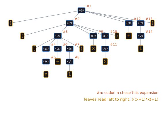
The codon numbers in the figure follow a depth-first, left-to-right walk of the derivation tree, which is the same order as a preorder traversal of a program tree. This is why each codon's meaning depends on all the earlier ones: the position of a codon in the genome does not say where in the program it acts, only how many expansions came before it.
Redundancy, wrapping and ripple
The modulo rule is many-to-one: with two productions, every even codon means the same thing. Changing codon 1 from 42 to 44 leaves the phenotype unchanged. O'Neill and Ryan (2001) describe this as a degenerate genetic code, after the biological term, and it is a source of neutral mutations.
Wrapping lets a short genome encode a longer derivation. Truncated to its first 10 codons, the genome above is incomplete without wrapping. With one wrap, the mapping reads 18 codons, eight of them a second time, and produces (((x+1)*x)-(x+1)): the same first eleven derivation steps, then different productions, because each reused codon is read against whatever nonterminal comes next, not the one it met the first time. Wrapping does not always succeed. The two-codon genome 0 1 never completes within ten wraps and is invalid.
Because every codon's meaning depends on all the choices before it, a change early in the genome propagates. Changing codon 2 from 118 to 119 turns the second <e> into <v>, every later codon is read against a different nonterminal, and the phenotype becomes (x-(1-(x+1))), which simplifies to $2x$. This propagation is often called a ripple effect. A change near the end can ripple as well: changing codon 13 from 75 to 76 produces (((x+1)*x)+(x-(x+1))), and the derivation now reads 22 codons, so it wraps.
The locality criticism
A representation has high locality when genotypes one mutation apart map to phenotypes that are also close. Rothlauf and Oetzel (2006) applied every single bit flip to 1,000 random GE genotypes of 160 bits, on the Santa Fe ant trail and on symbolic regression, and measured the tree edit distance between parent and offspring phenotypes. Most bit flips, about 82 percent on the ant trail and 94 percent on symbolic regression, left the phenotype unchanged. Of the flips that did change it, about 78 percent and 45 percent respectively produced a phenotype one edit away, and the rest could produce a very different program. In a comparison of $(1+1)$ evolutionary algorithms, mutation through the GE mapping performed worse than mutation applied directly to trees, although the authors note that low locality also made it easier to escape local optima. (These figures are from the working-paper version of the study.)
The script runs a smaller version on the grammar above: 30 random 20-codon genotypes whose phenotype contains at least one operator, with up to ten wraps. The median proportion of bit flips that leave the phenotype unchanged is 0.85 (interquartile range 0.80 to 0.92), partly because the median genotype reads only 10 of its 20 codons and the rest are neutral by construction. Counting only flips in codons that are read, the median is 0.70 (0.69 to 0.73), and the modulo rule explains why. For a rule with two productions only the lowest bit of the codon matters, so seven of its eight bit flips are neutral; for a rule with three productions every flip changes the choice, because no power of two is divisible by 3. Structured grammatical evolution, which ties each gene to one nonterminal, was designed to raise locality and reduce redundancy, and its authors report better performance than standard GE on several benchmark problems (Lourenço, Pereira, and Costa, 2016).
Stack-based GP and Push
A fourth family executes programs on a stack. Stack-based GP predates Push (Perkis, 1994), but the most developed system is Push, a language designed for evolving programs (Spector and Robinson, 2002). A Push program is a sequence of literals and instructions. A literal is pushed onto the stack for its type, and an instruction takes its arguments from the top of the relevant stacks and pushes its result. There is a separate stack for each type, such as integers, floats and booleans, so an instruction always receives arguments of the right type. An instruction that finds too few arguments on its stack does nothing, which makes every sequence of instructions a runnable program, and every mutation or crossover yields a valid offspring.
Worked example
Let the instruction x push the input onto the float stack. The postfix program x 1.0 FLOAT.+ x FLOAT.* 1.0 FLOAT.+ runs as follows at $x = 2$:
| Item | Float stack after |
|---|---|
x |
2 |
1.0 |
2, 1 |
FLOAT.+ |
3 |
x |
3, 2 |
FLOAT.* |
6 |
1.0 |
6, 1 |
FLOAT.+ |
7 |
The result is the top of the float stack, 7. Now insert noise: FLOAT.* x 1.0 FLOAT.+ TRUE x BOOLEAN.NOT FLOAT.* 1.0 FLOAT.+ FLOAT.-. The first FLOAT.* meets an empty float stack and does nothing. TRUE and BOOLEAN.NOT work on the boolean stack and do not disturb the floats. The final FLOAT.- finds a single float and does nothing. The program still computes $x^2 + x + 1$ at every test point. The no-op rule and the typed stacks give Push its own neutrality: code that is executed but has no effect.
Push also treats code as data: programs can manipulate pieces of code on a code stack and then execute them, so loops and recursion can evolve without being built into the representation. Spector and Robinson (2002) used this for autoconstructive evolution, in which programs construct their own offspring. Push3 made execution itself a stack, the exec stack, which evolved programs can manipulate (Spector, Klein, and Keijzer, 2005). PushGP, the GP system built on Push, became a common platform for general program synthesis. Helmuth and Spector (2015) assembled a suite of 29 benchmark problems taken from introductory programming exercises to test such systems.
Comparing the four
| Representation | Genotype | Non-coding material | What a small change can do |
|---|---|---|---|
| Linear GP | List of register instructions | Structural and semantic introns | Changing a destination or operand register can connect or disconnect whole blocks of instructions |
| Cartesian GP | Fixed-length list of integers | Inactive nodes | One output or connection gene can activate or deactivate many nodes |
| Grammatical evolution | Variable-length list of codons | Unread codons; redundant codon values | A change in an early codon can alter the meaning of every later codon |
| Push | List of literals and instructions | No-op instructions; values left unused on stacks | An inserted instruction shifts what later instructions find on the stacks |
All four have a large supply of neutral mutations, and all four allow some single mutations to make large changes. CGP's inactive nodes and LGP's structural introns can be identified from the genotype without running the program; whether a Push instruction is a no-op depends on the stack contents when it runs.
Human-competitive results
GP's most cited claim to practical success is Koza's (2010) survey of human-competitive results. Koza calls a result human-competitive if it satisfies at least one of eight criteria, among them that it would qualify as a patentable invention or improves on a patented one, that it equals or betters a result published as new in a peer-reviewed journal, and that it holds its own in a regulated competition against human contestants. He lists 76 instances that he was aware of, in fields from analog circuits and antennas to quantum computing, sorting networks and software repair. He observes that many used a developmental process and a representation native to the engineering field concerned, and that the production of such results has broadly tracked the growth of computing power.
The list should be read for what it is. It is one author's compilation, and the classification of each result rests on Koza's or the original authors' judgment; only those that later won awards were judged by a panel. It records successes, not attempts, so it cannot say how often GP succeeds on problems of a given kind. Several of the results duplicate the function of previously patented inventions. Koza notes that most of these were new designs rather than copies of the patented ones, but a problem that humans had already solved and specified is a different test from an open one.
Since 2004, the Human-Competitive Awards, or Humies, held at the annual Genetic and Evolutionary Computation Conference (GECCO), have offered cash prizes for such results (Koza, 2010; Human-Competitive Awards, 2026). Entries are judged by a panel, and they are open to any form of genetic and evolutionary computation, not only GP. Of the 76 results in Koza's table, 31 had received a Humies award. The criteria have since been condensed: the call for the 2027 awards lists four, and adds that the result must be described in enough detail to be independently reproduced (Human-Competitive Awards, 2026).
Relation to modern program synthesis
GP was among the first general methods for program synthesis, constructing programs from a specification, usually input-output examples. Recent systems keep the evolutionary loop but replace random variation with a large language model. In FunSearch (Romera-Paredes et al., 2024), a pretrained language model is prompted with high-scoring programs from a database and proposes new ones, an automated evaluator scores them, and the good ones join the database for later prompts. Applied to the cap set problem in combinatorics, it found constructions larger than the best previously known, and it also found bin-packing heuristics that improved on widely used baselines. AlphaEvolve (Novikov et al., 2025) extends the approach from single functions to whole code files and a wider range of problems, as described in AlphaEvolve and LLM-guided evolution.
In the terms of this article, the language model is a variation operator. Source text has very low locality under random character changes, but the model proposes edits that are usually syntactically valid and often meaningful, the property that GE's grammar, Push's no-op rule and CGP's fixed graph each secure in a more limited way. The rest of the loop is GP's: a population or archive of programs, selection by an automated evaluator, and many generations. The history of evolutionary computation traces the idea of evolving programs back to Friedberg's experiments in the 1950s.
References
- Brameier, M., and Banzhaf, W. (2007). Linear Genetic Programming, chapters 2 and 3. Springer.
- Eiben, A. E., and Smith, J. E. (2015). Introduction to Evolutionary Computing, 2nd ed., chapter 6. Springer.
- Helmuth, T., and Spector, L. (2015). General program synthesis benchmark suite. In Proceedings of GECCO 2015, 1039–1046. ACM.
- Human-Competitive Awards (2026). Call for entries: 24th annual (2027) Humies awards. human-competitive.org.
- Koza, J. R. (2010). Human-competitive results produced by genetic programming. Genetic Programming and Evolvable Machines, 11(3–4), 251–284.
- Lourenço, N., Pereira, F. B., and Costa, E. (2016). Unveiling the properties of structured grammatical evolution. Genetic Programming and Evolvable Machines, 17(3), 251–289.
- Miller, J. F. (2011). Cartesian genetic programming. In J. F. Miller (Ed.), Cartesian Genetic Programming, chapter 2, 17–34. Natural Computing Series, Springer.
- Miller, J. F., and Harding, S. L. (2008). Cartesian genetic programming (tutorial). In Proceedings of the GECCO 2008 Conference Companion, 2701–2726. ACM.
- Miller, J. F., and Thomson, P. (2000). Cartesian genetic programming. In Genetic Programming: Proceedings of EuroGP 2000, Lecture Notes in Computer Science 1802, 121–132. Springer.
- Novikov, A., Vũ, N., Eisenberger, M., Dupont, E., Huang, P.-S., Wagner, A. Z., Shirobokov, S., Kozlovskii, B., Ruiz, F. J. R., Mehrabian, A., Kumar, M. P., See, A., Chaudhuri, S., Holland, G., Davies, A., Nowozin, S., Kohli, P., and Balog, M. (2025). AlphaEvolve: A coding agent for scientific and algorithmic discovery. arXiv:2506.13131.
- O'Neill, M., and Ryan, C. (2001). Grammatical evolution. IEEE Transactions on Evolutionary Computation, 5(4), 349–358.
- Perkis, T. (1994). Stack-based genetic programming. In Proceedings of the First IEEE Conference on Evolutionary Computation, 148–153. IEEE.
- Romera-Paredes, B., Barekatain, M., Novikov, A., et al. (2024). Mathematical discoveries from program search with large language models. Nature, 625, 468–475.
- Rothlauf, F., and Oetzel, M. (2006). On the locality of grammatical evolution. In Genetic Programming: Proceedings of EuroGP 2006, Lecture Notes in Computer Science 3905, 320–330. Springer. Working-paper version: University of Mannheim, Working Paper 11/2005.
- Ryan, C., Collins, J. J., and O'Neill, M. (1998). Grammatical evolution: Evolving programs for an arbitrary language. In Genetic Programming: Proceedings of EuroGP 1998, Lecture Notes in Computer Science 1391, 83–96. Springer.
- Spector, L., Klein, J., and Keijzer, M. (2005). The Push3 execution stack and the evolution of control. In Proceedings of GECCO 2005, 1689–1696. ACM.
- Spector, L., and Robinson, A. (2002). Genetic programming and autoconstructive evolution with the Push programming language. Genetic Programming and Evolvable Machines, 3(1), 7–40.