The second assignment in CSC 742 asked for a genetic algorithm with a binary representation, applied to four of the test functions Kenneth De Jong used in his 1975 dissertation. Each variable was to be encoded as a bit string, decoded linearly into its interval, and evolved with fitness-proportionate selection, one- or two-point crossover with probability 0.9, and bit-flip mutation at rate $1/L$, where $L$ is the chromosome length. The runs used a population of 20 for 50 generations, plotted the best and average fitness per generation, compared 8-bit and 16-bit encodings, and ranked the functions from easiest to hardest. This article describes what I submitted, relates the assignment's versions of the functions to De Jong's originals, and extends the study by rerunning the same algorithm over thirty seeds to see which of the conclusions hold across repeated runs.
De Jong's five functions
De Jong (1975, appendix A) assembled an "environment" of five functions, all to be minimized, chosen to cover continuous and discontinuous, convex and non-convex, unimodal and multimodal, low- and high-dimensional cases, and one with noise. Each was restricted to a box and discretized so that the number of points on each axis was a power of two, so that each axis maps exactly onto the values of a binary string.
| Function | $n$ | Domain | Points per axis | Minimum | |
|---|---|---|---|---|---|
| F1 | $\sum_{i=1}^{3} x_i^2$ | 3 | $[-5.12, 5.12]$ | 1,024 | 0 at the origin |
| F2 | $100(x_1^2 - x_2)^2 + (1 - x_1)^2$ | 2 | $[-2.048, 2.048]$ | 4,096 | 0 at $(1, 1)$ |
| F3 | $\sum_{i=1}^{5} \lfloor x_i \rfloor$ | 5 | $[-5.12, 5.12]$ | 1,024 | $-30$ |
| F4 | $\sum_{i=1}^{30} i\, x_i^4 + \mathrm{Gauss}(0, 1)$ | 30 | $[-1.28, 1.28]$ | 256 | 0 without noise |
| F5 | Shekel's foxholes (below) | 2 | $[-65.536, 65.536]$ | 131,072 | about 1 |
F1 is a three-dimensional paraboloid. F2 is Rosenbrock's function (Rosenbrock, 1960), whose minimum lies at the end of a long, curved parabolic valley along $x_2 = x_1^2$, a feature of its fitness landscape that slows methods which follow the steepest slope. F3 is a five-dimensional step function, piecewise constant, a test of how a method handles discontinuities. F4 is a 30-dimensional quartic with Gaussian noise added to every evaluation. F5, which De Jong built following a suggestion of Shekel's, is
$$\frac{1}{F5(\mathbf{x})} = \frac{1}{500} + \sum_{j=1}^{25} \frac{1}{j + \sum_{i=1}^{2} (x_i - a_{ij})^6},$$
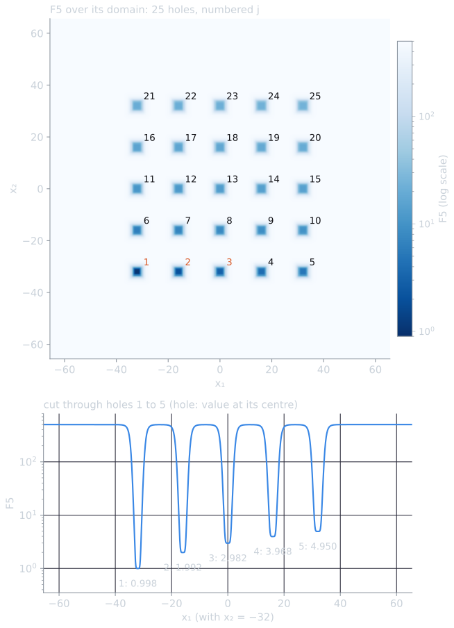
where the 25 points $(a_{1j}, a_{2j})$ form a $5 \times 5$ grid with coordinates in $\{-32, -16, 0, 16, 32\}$, with $a_{1j}$ running through the five values and $a_{2j}$ stepping up once every five holes. The surface is nearly flat at about 500, with 25 narrow holes whose bottoms take values close to 1 to 25, so F5 is the one multimodal function in the set.
The formula is easier to read term by term. Far from every hole, all the terms of the sum are tiny, the right-hand side is close to $1/500$, and F5 is close to 500 (499.98 at $(0, 50)$, for instance). At the centre of hole $j$ the $j$-th term is $1/j$, so F5 is a little below $j$: the other holes' terms add slightly to the sum. The sixth power makes the holes steep-sided and flat-bottomed: one unit away from a centre the term has fallen from $1/j$ to $1/(j + 1)$, and two units away to $1/(j + 64)$. The script computes 0.998 at the centre of hole 1, $(-32, -32)$, 1.992 at hole 2, and 23.81 at hole 25, where the influence of the other 24 holes is largest.
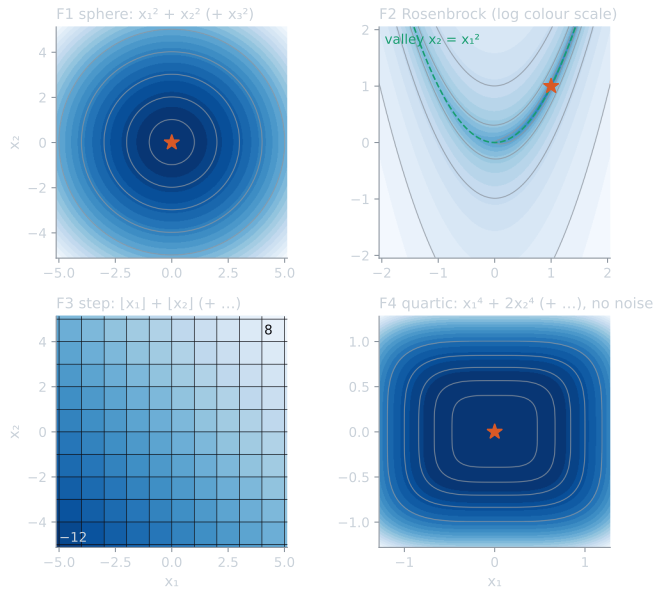
The assignment specified four of these, under its own names and with some changes, and the submission implemented them as specified. Its "Sphere Model" is F1. Its "Weighted Sphere Model" has the formula of F2, Rosenbrock's function, whose difficulty comes from the curved valley rather than from unequal weights on the axes, as the name might suggest. Its step function used $n = 4$, so its minimum is $4 \cdot \lfloor -5.12 \rfloor = -24$, not $-30$. Its "Noisy Quartic" used $n = 4$ instead of 30, and uniform noise on $[0, 1)$ instead of Gaussian noise with mean 0 and variance 1. F5 was not included, so the comparison has no multimodal function.
The submitted algorithm
The program (binary_ga.py) encoded each variable in $b$ bits, most significant first, and decoded the integer value $k$ of each substring as
$$x = L + \frac{U - L}{2^b - 1}\, k,$$
so the grid spacing is $(U - L)/(2^b - 1)$: 0.0402 for 8 bits and 0.000156 for 16 bits on $[-5.12, 5.12]$. The chromosome lengths ranged from $L = 16$ (Rosenbrock, 8 bits) to $L = 64$ (step and quartic, 16 bits).
The best 8-bit sphere solution of the report shows the decoding at work. Its 24-bit chromosome is three 8-bit genes:
| Gene | Bits | $k$ | $x = -5.12 + 0.040157\,k$ |
|---|---|---|---|
| $x_1$ | 10000010 | 130 | +0.1004 |
| $x_2$ | 10000011 | 131 | +0.1405 |
| $x_3$ | 01111101 | 125 | −0.1004 |
(The figure script computes these; the report printed the values to three decimals.) The two grid points nearest zero are $k = 127$, 01111111, at $-0.0201$, and $k = 128$, 10000000, at $+0.0201$. The first and third genes decode to the same distance from zero on opposite sides, and since $130 + 125 = 255$ their bit strings are exact complements: they differ in all eight bits, a first sign of the Hamming cliffs discussed below.
Selection was a roulette wheel on the transformed value $1/(f + 1)$, which turns minimization into maximization; for the step function, whose values can be negative, the population's values were first shifted so that the smallest became 1. Each pair of parents came from two independent spins. Two-point crossover was applied with probability 0.9 and bit-flip mutation at rate $1/L$, and the offspring replaced the whole population, with no elitism. The program reported the best individual evaluated in any generation. Its line setting a random seed was left commented out, so the submitted runs cannot be regenerated exactly.
The submitted results
Each function and encoding was run once. The report's table:
| Function | Bits | Best value | Best solution |
|---|---|---|---|
| Sphere | 8 | 0.0399 | (0.100, 0.141, −0.100) |
| 16 | 0.0104 | (0.085, 0.007, −0.056) | |
| Rosenbrock | 8 | 0.2866 | (1.036, 1.020) |
| 16 | 0.0641 | (0.792, 0.641) | |
| Step ($n = 4$) | 8 | −23 | (−5.04, −4.96, −5.12, −5.08) |
| 16 | −23 | (−5.04, −4.80, −5.04, −5.11) | |
| Noisy quartic ($n = 4$) | 8 | 0.0321 | (−0.356, 0.015, 0.236, 0.075) |
| 16 | 0.0139 | (0.292, −0.045, 0.036, 0.091) |
The decoded points are consistent with the values. For example, $0.100^2 + 0.141^2 + 0.100^2 = 0.0399$, and the step solution has floors $-6, -5, -6, -6$, one variable short of the minimum. From this table the report concluded that 16 bits gave better or equal results on every function, that the Rosenbrock result improved by a factor of 4.5 with the longer encoding, and that the functions ranked from easiest to hardest as sphere, quartic, step, Rosenbrock.
Thirty seeds
To see how much of that table is the algorithm and how much is the draw of random numbers, I ported the program's operators unchanged into tools/experiments/evolution/dejong_ga.py in the site repository and ran each function and encoding with seeds 0 to 29. The table gives the median and interquartile range of the best value found, the range over all thirty runs, and the best value the grid can represent at all.
| Function | Bits | Grid floor | Median [IQR] | Min to max |
|---|---|---|---|---|
| Sphere | 8 | 0.0012 | 0.0077 [0.0044, 0.0109] | 0.0012 to 0.101 |
| 16 | $1.8 \times 10^{-8}$ | 0.0058 [0.0028, 0.0131] | 0.0002 to 0.045 | |
| Rosenbrock | 8 | 0.0016 | 0.053 [0.013, 0.207] | 0.0016 to 1.22 |
| 16 | $2.6 \times 10^{-8}$ | 0.125 [0.031, 0.351] | $2.4 \times 10^{-6}$ to 2.95 | |
| Step ($n = 4$) | 8 | −24 | −23 [−24, −23] | −24 to −22 |
| 16 | −24 | −23 [−24, −23] | −24 to −22 | |
| Noisy quartic ($n = 4$) | 8 | 0 + noise | 0.031 [0.016, 0.043] | 0.0029 to 0.086 |
| 16 | 0 + noise | 0.037 [0.021, 0.054] | 0.0021 to 0.087 |
Every value in the submitted table lies inside the range of the thirty reruns for its row. To compare the encodings directly, the script computes the Vargha and Delaney (2000) $A$ statistic: the probability that a randomly chosen 16-bit run ends lower than a randomly chosen 8-bit run, counting ties as one half. A value of 0.5 means no difference. The values are 0.52 for the sphere, 0.39 for Rosenbrock, 0.49 for the step function, and 0.42 for the quartic. Under the assignment's budget the 16-bit encoding is no better on any of the four functions, and on Rosenbrock it is somewhat worse.
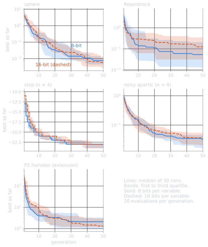
The report plotted one curve per function and encoding. The same plot over thirty runs, the median and the middle half of the best value found so far, shows how the runs got there:
| Function | Bits | Generation 1 | 10 | 25 | 50 |
|---|---|---|---|---|---|
| Sphere | 8 | 4.20 | 0.196 | 0.0270 | 0.0077 |
| 16 | 4.23 | 0.179 | 0.0246 | 0.0058 | |
| Rosenbrock | 8 | 3.62 | 0.139 | 0.0751 | 0.0533 |
| 16 | 2.31 | 0.295 | 0.201 | 0.125 | |
| Step | 8 | −13 | −21 | −22 | −23 |
| 16 | −11 | −20 | −22 | −23 | |
| Noisy quartic | 8 | 0.950 | 0.157 | 0.0481 | 0.0314 |
| 16 | 0.868 | 0.136 | 0.0576 | 0.0367 |
The table gives the medians plotted in the figure, rounded to three significant figures; the figures are drawn, and the medians computed, by tools/figures/de-jong-test-functions-ga.py. On the sphere, the median falls by a factor of about 20 in the first ten generations and only by a factor of about 3.5 over the last 25. On the step function, the median reaches −21 or −20 by generation 10 and then gains one level at a time, each gain requiring one more variable to reach the bottom step, $\lfloor x_i \rfloor = -6$, which covers only $[-5.12, -5)$, about 1% of each variable's range. The runs slow down long before the budget ends, the stall that the section on selection below explains.
What repeated runs reveal
The single runs were enough to show that the implementation worked. Every rerun ended far below the value of a typical random point, which De Jong (1975, appendix A) gives as 26.2 for F1 and 494 for F2 averaged over the domain, and the curves had the qualitative shapes the report described, with plateaus and integer jumps on the step function and large swings in the average on Rosenbrock, where a single offspring off the valley floor can score in the hundreds.
A difference between encodings needs many runs. On Rosenbrock the thirty 8-bit runs span three orders of magnitude, from 0.0016 to 1.22. Two runs drawn from such a distribution can differ by a factor of 4.5 with the same encoding, so a factor of 4.5 between one 8-bit run and one 16-bit run cannot by itself separate the encodings. Over thirty runs, the report's conclusion that 16 bits helped on the continuous functions is not borne out: the medians favor 8 bits on two of the three. The report's expectation of minimal variance between runs on the sphere can now be checked as well: the thirty 8-bit sphere runs range from 0.0012 to 0.101.
Ranking the functions by difficulty needs a common scale. The best values are on different scales: a Rosenbrock value of 0.05 and a sphere value of 0.05 are not equally good, and a step value of $-23$ is not comparable to either. A ranking needs a common measure, such as the fraction of runs that reach a fixed tolerance of the optimum or the number of evaluations needed to get there, and enough runs to estimate it (Eiben and Smith, 2015, ch. 9), compared with the kind of care described in significance testing. On the step function, for instance, the reruns reach the minimum of $-24$ in 14 of 30 runs with 8 bits and 12 of 30 with 16 bits. The one function that might have upset the ranking, the multimodal F5, was not in the set; I run it below.
The noisy quartic's "best value" partly reflects the noise. The program kept the lowest value ever evaluated, and each evaluation added a fresh uniform draw from $[0, 1)$, whose mean is 0.5. Over 1,000 evaluations the minimum is selected partly for a small noise draw. In the reruns, the noise in the reported best value has a median of 0.010 (8 bits) and 0.012 (16 bits), against an expected 0.5, and the noise-free quartic of the same individual has a median of 0.013 and 0.018. The noise draw and the quality of the solution contribute comparable amounts to the reported value. With De Jong's Gaussian noise the effect would be stronger, since the reported minimum would typically be negative. A fairer report gives the noise-free value when, as here, the noise-free function is known, or else the average of several fresh evaluations of the final candidate; averaging repeated evaluations is a standard remedy for noisy fitness (Eiben and Smith, 2015, ch. 11).
Why sixteen bits did not help
Precision was not what limited these runs. With 8 bits on $[-5.12, 5.12]$ the two grid points nearest zero are $\pm 0.0201$, so no 8-bit sphere solution can score below $3 \times 0.0201^2 = 0.0012$. The median 8-bit run ended at 0.0077, more than six times that floor, and 7 of the thirty runs reached it. A finer grid lowers a floor that the search was not reaching. Meanwhile the 16-bit chromosome is twice as long, so the same 1,000 evaluations explore a far larger space, and at rate $1/L$ mutation still flips about one bit per offspring. Half the time that bit is among the eight low-order bits of a variable, and flipping it moves the decoded value by less than 0.04 on $[-5.12, 5.12]$.
Selection also weakens as the run proceeds. The transform $1/(f + 1)$ is nearly 1 for every value of $f$ close to 0: an individual at $f = 0.005$ gets 0.995 and one at $f = 0.5$ gets 0.667, so the best is chosen only 1.5 times as often as an individual a hundred times worse. For a whole population, take twenty individuals: one at $f = 0.005$, nine at 0.05 and ten at 0.5. Their weights are 0.995, 0.952 and 0.667, which sum to $0.995 + 9 \times 0.952 + 10 \times 0.667 = 16.23$, so each spin picks the best with probability $0.995 / 16.23 = 0.061$, and twenty spins give it 1.23 copies on average, barely more than the one copy every individual would get by chance. In the last generation of the sphere runs, the best individual's expected number of copies under the roulette wheel had a median of 1.78 (8 bits) and 1.43 (16 bits), against 1.0 under uniform random choice. Eiben and Smith (2015, ch. 5) describe this loss of selection pressure when fitness values are close together as a known weakness of fitness-proportionate selection; the cures they discuss include scaling, ranking and tournament selection, covered in selection pressure and premature convergence. Without elitism the population can also lose its best individual, which the program kept only in its record of the best so far.
De Jong saw a related stall in his own experiments. In a single run of his basic plan on F1, the population had effectively converged in 25 of its 30 bit positions by trial 3,000, and his performance measures improved little or not at all from then on, with the better of them stuck at 0.018 rather than the minimum of zero, because crossover can produce only points whose bit values are all still present somewhere in the population (De Jong, 1975, ch. 3). His performance curves, as he noted, were averaged over independent runs.
The binary code itself adds a small oddity. On a symmetric domain with an even number of grid points, zero falls exactly between the integers $2^{b-1} - 1$ and $2^{b-1}$, which are 01111111 and 10000000 for 8 bits and differ in every bit. Crossing the optimum from one side to the other in a single step therefore takes a change in all eight bits. Gray codes remove such Hamming cliffs between adjacent integers.
The function the assignment left out
The assignment had no multimodal function, so its comparison could not show the failure that populations are meant to guard against: settling in a local optimum. To see what the same algorithm does on one, I added De Jong's F5 to the rerun script, decoded onto $[-65.536, 65.536]$ with the same operators, population, budget and seeds. It is an extension of the study, not part of what I submitted.
| Bits | Best value, median [IQR] | Runs at the global minimum, 0.998 | Runs ending nearest each hole (hole: runs) |
|---|---|---|---|
| 8 | 2.11 [0.998, 3.33] | 11 of 30 | 1: 19, 2: 8, 3: 2, 4: 1 |
| 16 | 1.32 [1.21, 2.98] | 6 of 30 | 1: 22, 3: 3, 4: 2, 6: 1, 9: 1, 11: 1 |
"Runs at the global minimum" counts best values below 0.999; the last column assigns each run's best point to the nearest hole centre. Three things stand out.
Most runs find the right hole, and many do not. The deepest holes, 1 to 5, lie along the bottom row, and every run but three ended in one of them. Eleven of the thirty 8-bit runs ended in hole 2, 3 or 4, whose bottoms are 1 to 3 units above the global minimum. With a population of 20 and the fading selection pressure described above, a run that finds a reasonable hole early tends to stay there: moving from hole 2 to hole 1 means crossing 16 units of plateau at about 500, and any single offspring that tries it scores a hundred times worse than its parents.
The plateau is what makes the start hard. The median best value in the first generation was 263 for 8 bits and 261 for 16, against 500 on the plateau: in most runs, at least one of the twenty random initial points already lies on the side of some hole. From there the median in the figure above drops by one to two orders of magnitude within ten generations, as soon as a few individuals sit in a hole. On the plateau itself, the values differ only in the third or fourth significant figure, and the roulette wheel cannot tell them apart.
Finer encoding means closer to, not at, the bottom. The 8-bit grid has a point 0.125 from the centre of hole 1 in each coordinate, and 11 runs reached that point exactly. The 16-bit runs got into hole 1 more often (22 against 19) and had the lower median, but only 6 reached 0.998 to three decimals; most of the other runs in hole 1 stopped between 1.2 and 1.6, a little off the centre in a hole whose floor is flat to the eye but still curved. As on the continuous functions, the extra precision was not what limited the search.
What I would change
- Run every configuration many times with recorded seeds, and report medians and spreads, as this article does.
- Add De Jong's original definitions alongside the assignment's versions, including $n = 5$ for F3, $n = 30$ and Gaussian noise for F4, and F5, so that the results can be compared with the literature.
- Measure difficulty on a common scale, by success rate at a tolerance or by evaluations to reach it.
- Keep the best individual (elitism of one) and replace the $1/(f + 1)$ roulette wheel with rank-based or tournament selection, so that selection pressure does not fade as the population improves.
- Report a noise-free or re-evaluated value for the noisy function.
- Test the encoding question with a larger budget than the assignment allowed. At 50 generations the 8-bit grid is not the bottleneck, so the question of how many bits to use only becomes interesting when the search can get close to the 8-bit floor.
References
- De Jong, K. A. (1975). An Analysis of the Behavior of a Class of Genetic Adaptive Systems, chapter 3 and appendix A. PhD dissertation, University of Michigan.
- Eiben, A. E., and Smith, J. E. (2015). Introduction to Evolutionary Computing, 2nd ed., chapters 5, 9 and 11. Springer.
- Rosenbrock, H. H. (1960). An automatic method for finding the greatest or least value of a function. The Computer Journal, 3(3), 175–184.
- Vargha, A., and Delaney, H. D. (2000). A critique and improvement of the CL common language effect size statistics of McGraw and Wong. Journal of Educational and Behavioral Statistics, 25(2), 101–132.