The final project in CSC 742 was open-ended. I chose to implement NEAT from scratch and use it to evolve simulated soft robots, body and brain together, in the Evolution Gym (EvoGym) benchmark. Each robot was a body of at most 5×5 voxels with a neural network controlling its muscles, and the task was EvoGym's simplest, Walker-v0: move right along flat ground as far as possible. The code is public at github.com/mdb42/evogym-playground, and the report and presentation describe the implementation stage by stage, with the best fitness each stage reached.
This article describes the project as submitted and reports its numbers as the report gives them. It then considers what kind of evidence those numbers are, one run per stage, and what a controlled experiment answering the project's questions would look like.
Evolving bodies and brains
Evolving a robot's body together with its controller goes back to Sims (1994), whose virtual creatures were built from blocks connected by joints. A directed-graph genotype described both the morphology and the neural circuitry that drove the joints, and selection for swimming, walking, jumping or following produced a variety of locomotion strategies. Later work replaced rigid blocks with soft material. Cheney, MacCurdy, Clune and Lipson (2013) evolved robots made of soft voxels in four materials, two passive and two that expand and contract periodically in opposite phase. The body was encoded by a compositional pattern-producing network evolved with NEAT (CPPN-NEAT). Selected for speed, these robots moved faster than robots evolved with a direct voxel-by-voxel encoding, and their shapes looked more natural. Control in that study was fixed: the muscle voxels actuated on a set periodic cycle, and only the body evolved.
When the controller is evolved as well, a further difficulty appears. A controller is tuned to the body it grew up in, so most changes to the body make the robot worse until the controller readapts. Cheney, Bongard, SunSpiral and Lipson (2018) argued that this coupling is a main reason body-brain co-optimization stalls, and proposed morphological innovation protection: temporarily reducing selection pressure on individuals whose bodies have just changed, so that their controllers have time to catch up. The same idea, protecting a new structure until it is tuned, is what NEAT's speciation does for new network structure (Stanley and Miikkulainen, 2002).
EvoGym and the Walker task
EvoGym (Bhatia et al., 2021) is a benchmark for co-designing soft robots. A robot is a grid of voxels, each empty, rigid, soft, a horizontal actuator or a vertical actuator, and the simulator models every voxel as a cross-braced square of springs in two dimensions. An actuator's action sets its target length, between 0.6 and 1.6 times its rest length. The benchmark offers more than 30 locomotion and manipulation tasks. Its baselines pair a body optimizer (a genetic algorithm, Bayesian optimization or CPPN-NEAT) with reinforcement learning (proximal policy optimization) that trains a controller for each proposed body. They use 5×5 bodies for most tasks, populations of 25 and at most 750 bodies per run, and average each result over 6 random seeds. The genetic algorithm did best overall, and all three failed on the hardest tasks.
In Walker-v0 the reward at each step is the distance the robot's center of mass moved to the right, in simulator units where a voxel is 0.1 wide, plus a one-time bonus of 1 for reaching the end of the terrain. The fitness of a robot is the total reward over an episode, so a fitness of 5 corresponds to a net movement of about 50 voxel widths.
The implementation
Each individual carried a body, a 5×5 integer grid, and a NEAT genome for its controller. Body and controller were evaluated together and inherited together, which the report calls single-population cooperative coevolution; there is no separate population of controllers to pair with bodies, as there would be in cooperative coevolution proper. The report describes the design as follows.
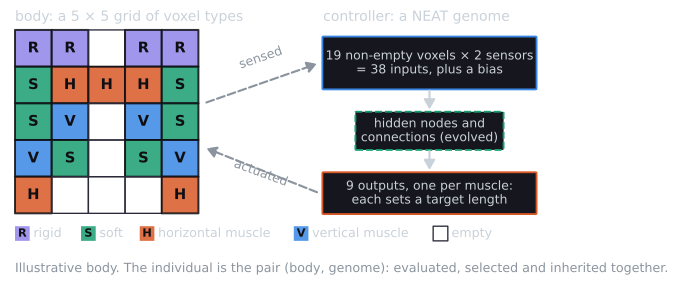
The figure shows why body and controller cannot be evolved independently here. The size of the controller's input and output layers is a function of the body, so every body mutation that adds or removes a voxel also changes what the controller must read and drive.
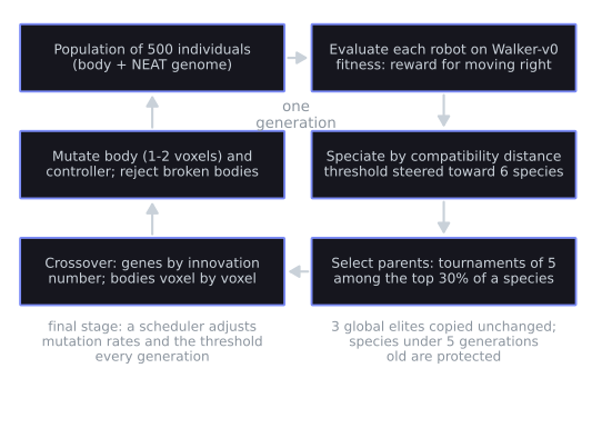
- Bodies. The initial bodies came from EvoGym's random sampler, which guarantees a connected body. A body mutation changed one or two voxels, the number drawn from a Poisson distribution whose rate is the morphology mutation rate. An empty position received a random voxel type, and an occupied one was removed or changed to another type with equal probability. A flood fill rejected bodies that fell into pieces, with up to 10 attempts before the original body was kept. Body crossover was uniform, voxel by voxel, under the same connectivity check.
- Controllers. Each non-empty voxel supplied two sensor inputs, there was a bias input, and each muscle voxel had one output. Instead of starting from minimal networks, the implementation connected input-output pairs with probability 0.8 and guaranteed every output at least one connection, so that no muscle started inactive. The mutations were weight perturbation or replacement, adding a connection (with a check against cycles), adding a node by splitting a connection, toggling a connection on or off, and changing a hidden node's activation among tanh, sigmoid, ReLU and identity.
- Changing bodies. When a body mutation added voxels, the genome gained input nodes, and each new muscle received an output node connected to the bias. When a body shrank, nothing was removed: the controller padded or truncated its input vector and ignored surplus outputs, so control patterns for lost parts stayed in the genome in case similar bodies returned.
- NEAT machinery. Genes carried innovation numbers, and crossover aligned them, taking unmatched genes from the fitter parent. Species were formed with the compatibility distance using $c_1 = c_2 = 1.0$ and $c_3 = 0.4$, and an initial threshold of 3.0, the values Stanley and Miikkulainen (2002) used in all their experiments except the hardest pole-balancing variant, with a population of 150. Here the threshold was adjusted every generation to steer toward six species, and species younger than five generations were protected from removal. Parents were chosen by tournaments of five among the top 30% of a species, with three global elites.
- Scale. The report gives a population of 500, 400 generations, and evaluation spread across CPU cores, which brought a run from days to hours.
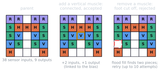
The connectivity check is a flood fill: start at any voxel, repeatedly visit non-empty neighbours that share an edge, and compare the number visited with the number of non-empty voxels. If they differ, the body has fallen into pieces.
Stage by stage
The project was built incrementally, and each stage was run and recorded. The report's table, with the stage descriptions from the report and presentation:
| Stage | What changed | Best fitness |
|---|---|---|
| Random control | Bodies evolve; every muscle receives a random action at every step | 3.68 |
| Neural network, mutation only | NEAT-style networks with 8 sensor inputs, tanh units, no crossover | 3.05 |
| With crossover | Crossover of networks by position in the gene list, uniform crossover of bodies | 3.26 |
| Protected niche evolution | Speciation by compatibility distance | 4.18 |
| Full sensation | Two inputs per voxel instead of 8 in total | 4.39 |
| Enable/disable, activation functions | Toggling connections; four activation functions | 5.14 |
| Dynamic parameter scheduling | The scheduler described below | 5.61 |
Each stage came with a recorded video, and the report describes what changed in behavior. Under random control, evolution found bodies with vertical muscles aligned in columns, which hop. Adding neural control lowered the best fitness while producing gaits that looked more coordinated; the report attributes the drop to the larger search space, since evolution now had to find a controller as well as a body. The first crossover, which aligned genes by position rather than by innovation number, produced robots with "functionless body mass grafted onto functional lower bodies".
The speciation stage gives the project's clearest observation. Early in that stage the best robot was a jumper with synchronized vertical muscles, at fitness 3.57. A robot with a shuffling, crawling gait scored only 1.17, but it sat in its own species, so it reproduced instead of being displaced by jumpers. Its descendants reached 4.18, the best result up to that point. That is the behavior speciation is designed to produce, and the run shows it happening.
With full sensation, the best robot moved with a rippling wave through its body. With connection toggling and the extra activation functions, the report describes the first bipedal gait. The report also mentions a preliminary experiment that began from much sparser networks. After 100 generations its robots had learned to roll after falling rather than walk, which the report treats as a deceptive local optimum and as support for the denser starting networks.
The scheduler run
The final stage added a scheduler that adjusted the parameters at every generation. As the report describes it, the scheduler worked in three fixed phases (exploration until generation 50, optimization until 150, fine-tuning after that) with progressively lower mutation rates. After 15 generations without a new best it multiplied the mutation rates by 1.5, and after 30 it raised them further and halved the compatibility threshold. It adjusted the threshold toward the target of six species, made the weight-mutation strength oscillate sinusoidally with a 25-generation period, and injected random individuals when the population seemed to have converged.
The fitness plot of that run shows the best fitness rising from about 0.7 to about 4.5 within roughly the first 30 generations. It then stays between about 4.6 and 4.8 until shortly before generation 300, climbs in steps to 5.61 by about generation 350, and stays there until the run ends at 400. The average fitness falls toward zero during the plateau. The species count swings between 1 and 29 and never settles at the target of six. The report reads the plateau as a failure of stagnation detection: any improvement, however small, reset the 15-generation counter, and the fixed phases kept mutation rates low regardless of progress. It reads the oscillation in species count as a control problem, with an adjustment too gentle to stop fragmentation and an emergency halving that overshot. Its proposed remedies are a minimum size for what counts as improvement, shorter stagnation windows, adjustment rates that scale with the distance from the target species count, and decoupling the fixed phases from the performance-based interventions.
Reading the results
Each row of the stage table is one run. The stages differ in code, possibly in settings, and in random seed, and no stage was repeated. The run-to-run spread of best fitness under a fixed configuration is unknown, so differences of 0.2, such as 3.05 to 3.26 or 4.18 to 4.39, cannot be attributed to the component that was added. Some may be. The stage table records the history of a growing implementation, and it is good evidence that the implementation worked, since the robots walk. It is not an ablation study. The report's conclusion that every component "proved essential" would need the components removed one at a time from the final system, with repeated runs, to support it.
The 52% improvement is measured against a morphology-only baseline. $(5.61 - 3.68)/3.68 = 0.524$, so the arithmetic is right. But 3.68 is the best body evolved for random actuation, not a neural controller with its training removed, and not the same system with one part disabled. It shows that the final system beat body evolution alone, in one run each.
The scheduler's effect is not isolated. The late climb came in a run whose scheduler changed many things at once, and the run is also the one the scheduler's design was judged on. Whether the climb is due to the scheduler, to one of its mechanisms, or to chance would take repeated runs with and without it.
The speciation observation is the strongest. It comes from within one stage's run rather than from a comparison between runs, so it does not depend on the run-to-run spread. It shows that protection let a low-fitness lineage survive and later overtake the leaders, which is the qualitative point the report makes.
A controlled follow-up
The project's three research questions can be answered with the same code, and the design follows from the points above.
- Fix and record the protocol. Save the full configuration of every run with its seed and results, and hold the evaluation settings and the budget of evaluations constant across conditions, so that any difference between conditions comes from the component being tested.
- Repeat every condition. One run per configuration cannot separate a design choice from luck. EvoGym's own baselines averaged 6 seeds per algorithm. Ten to thirty runs per condition, reported as median and interquartile range with an effect size, as in the De Jong rerun, would show how large the run-to-run spread is before any component is credited.
- Ablate from a common base. Remove one component at a time from the final system (speciation, crossover, full sensation, activation diversity, the scheduler) under an equal budget of evaluations, rather than adding them in sequence with other changes in between.
- Use baselines that isolate body and brain. Body evolution with random actuation; a fixed hand-designed walker with an evolved controller; evolved bodies with an open-loop periodic actuation like that of Cheney et al. (2013). These say how much each half contributes.
- Test protection directly. Bodies changed by mutation throughout the run, which is the situation Cheney et al. (2018) studied. Comparing speciation with their morphological innovation protection, or with both, would test the project's second question head-on.
What I take from it
The project met its main aim: a working NEAT, written from scratch, evolved bodies and controllers together and produced robots that walk. Its clearest finding is the protected crawler lineage. Its most useful lesson is about evidence. A sequence of single runs, each with new code, can show that an implementation works and suggest where to look, but it cannot rank the components. The same is true of a scheduler with many interacting mechanisms tuned on the run it is judged by. The code is public, which makes a controlled follow-up straightforward to set up.
References
- Bhatia, J., Jackson, H., Tian, Y., Xu, J., and Matusik, W. (2021). Evolution Gym: A large-scale benchmark for evolving soft robots. In Advances in Neural Information Processing Systems 34, 2201–2214.
- Cheney, N., Bongard, J., SunSpiral, V., and Lipson, H. (2018). Scalable co-optimization of morphology and control in embodied machines. Journal of the Royal Society Interface, 15(143), 20170937.
- Cheney, N., MacCurdy, R., Clune, J., and Lipson, H. (2013). Unshackling evolution: Evolving soft robots with multiple materials and a powerful generative encoding. In Proceedings of the 15th Annual Conference on Genetic and Evolutionary Computation (GECCO '13), 167–174.
- Sims, K. (1994). Evolving virtual creatures. In Proceedings of the 21st Annual Conference on Computer Graphics and Interactive Techniques (SIGGRAPH '94), 15–22.
- Stanley, K. O., and Miikkulainen, R. (2002). Evolving neural networks through augmenting topologies. Evolutionary Computation, 10(2), 99–127.