Take 240 individuals and a budget of 60,000 fitness evaluations, and use them in two ways. In one, the 240 form a single population in which any individual can be selected against and mated with any other. In the other, they are split into 8 groups of 30, each running its own genetic algorithm, and every few generations each group sends copies of its two best members to a neighbouring group. Run both on Rastrigin's function in 10 variables, 30 times each. The single population ends with a median best value of 0.24 and never reaches the global optimum. The divided population, migrating every 5 generations around a ring, reaches the optimum in 29 of 30 runs.
The divided version is an island model, also called a multi-deme or coarse-grained genetic algorithm. Each subpopulation, or deme, is an island; the occasional exchange of individuals is migration. Island models were developed largely with parallel computers in mind, one island per processor, and most research on parallel genetic algorithms has concentrated on them (Cantú-Paz, 1998). They are also used on a single processor, because dividing the population changes the search, not only its speed. This article describes the design choices, what migration does to diversity, the classic experiments, and the related cellular model, which divides the population more finely still. Parallelizing evaluation alone, without changing the algorithm, is the subject of master-slave parallel evaluation.
A parallel model, not only a parallel implementation
A simple genetic algorithm is panmictic: selection compares every individual with every other, and any two can mate. An island model restricts both to the island. That makes it a different algorithm, a parallel model in the terms of Alba and Tomassini (2002), whether its islands run on 8 processors or on one. Eiben and Smith (2015, ch. 5) treat island models, together with the cellular models described below, as implicit methods for preserving diversity, alongside explicit methods such as fitness sharing and crowding (see selection pressure and premature convergence).
The reasoning is the following. A small population converges quickly, by selection and by drift, and it converges somewhere that depends on its starting point and its luck. Several small populations converge to several different places. Each may be a local optimum, but they are probably different local optima, holding different partial solutions. Migration then lets those partial solutions meet, and crossover can combine them. The single large population, by contrast, settles on one region, and once its diversity is spent, crossover has nothing new to combine.
Design choices
An island model adds a set of parameters to those of the genetic algorithm running on each island.
- Number and size of islands. Usually equal, with the total population fixed.
- Migration size, or rate: how many individuals move in each migration event, as an absolute number or as a fraction of the deme.
- Migration interval, also called the epoch length: how many generations pass between migrations. Migration can also be triggered by events, such as an island's diversity falling below a threshold.
- Migration policy: which individuals emigrate (the best, or random ones) and which ones the immigrants replace at the destination (the worst, or random ones). Migrants may be copies, leaving the source unchanged, or may move.
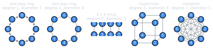
- Topology: which islands send to which. Common choices are a unidirectional or bidirectional ring, a two-dimensional grid or torus, a hypercube, a fully connected graph, and random topologies that draw new connections at every migration event. A topology's degree is the number of islands each island receives from.
- Synchrony: whether all islands migrate at the same moment, or each sends and receives on its own schedule, as happens naturally on processors running at different speeds.
These parameters are not independent. Migrating 2 individuals every generation and 10 every 5 generations move the same number of individuals, but they do not have the same effect.
Two numbers summarize a topology for the purposes of this article. Its degree says how many sources an island hears from at each migration event, and so how quickly its own composition is diluted. Its diameter, the largest number of hops needed to get from any island to any other along the links, says how many migration events a good individual needs to reach every island. With 8 islands:
| Topology | Degree | Diameter | Migrants received per event (one per link) |
|---|---|---|---|
| One-way ring | 1 | 7 | 1 |
| Two-way ring | 2 | 4 | 2 |
| $2 \times 4$ torus | 3 | 3 | 3 |
| Hypercube (3 dimensions) | 3 | 3 | 3 |
| Complete | 7 | 1 | 7 |
(The $2 \times 4$ torus has degree 3 rather than 4 because, with only two rows, an island's neighbours above and below are the same island.) A two-dimensional torus of $k \times k$ islands has diameter $2\lfloor k/2 \rfloor$ and a hypercube of $2^d$ islands has diameter $d$, so for large numbers of islands both grow far more slowly than the diameter $m - 1$ of a one-way ring of $m$ islands. The cost is in messages: every island talks to more neighbours.
What migration does to diversity
Migration pulls in two directions. It spreads good material between islands, which is the reason for having it. It also makes the islands more alike, which undoes the reason for dividing the population in the first place. With very frequent migration the islands behave much like one panmictic population; with none, they are independent runs of a smaller genetic algorithm.
Migration also changes selection pressure. When the best individuals emigrate and replace the worst at the destination, selection on fitness has acted twice, once at each end. Cantú-Paz (2000) identifies best-replaces-worst as the strongest of the four combinations of emigrant choice and replacement, and notes that it is the one most commonly used. Whitley, Rana, and Heckendorn (1999) observed the same effect in exact infinite-population models: migration of the best strings increased selection for fitness, and in their example made the islands converge faster.
Skolicki and De Jong (2005) studied the two basic migration parameters systematically on a suite of test functions, with a random topology. The migration interval turned out to be the dominant factor, with migration size generally playing a minor role in the quality of the best solution found. Even small migrations had a marked effect, comparable to that of larger ones. Measurements of genetic diversity showed why very frequent migration hurt: islands came to dominate one another, and the population lost its global diversity before the islands could exchange solutions that would combine into better ones. Rare migration hurt too, by slowing convergence.
Takeover in structured populations
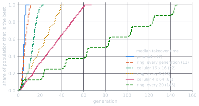
The speed with which a good individual spreads is measured by the takeover time, the number of generations selection alone needs to fill the population with copies of the best individual (Goldberg and Deb, 1991; see selection pressure). Population structure lengthens it. The second part of tools/experiments/evolution/island_model.py in the site repository measures takeover with 256 individuals, one of them better than the rest and no variation at all. In every generation each individual's slot holds a binary tournament among its neighbours and takes the winner if it is fitter. Only the definition of the neighbourhood changes. For 8 islands of 32, the neighbourhood is the individual's own island, and every $\tau$ generations each island sends a copy of its best member to the next island on a ring. Medians over 30 seeds:
| Population structure | Takeover time (generations) |
|---|---|
| Panmictic | 7 |
| 8 islands of 32, ring, migration every generation | 11 |
| 8 islands of 32, ring, every 5 generations | 40 |
| 8 islands of 32, ring, every 20 generations | 145 |
The panmictic figure can be derived. Let $q_t$ be the share of slots not yet holding the best individual after $t$ generations. A slot that does not hold it acquires it if either of its two tournament draws is the best, which happens with probability $1 - q_t^2$, so it stays without it with probability $q_t^2$. In a very large population the unfilled share therefore evolves as
$$q_{t+1} = q_t \cdot q_t^2 = q_t^3, \qquad q_t = q_0^{\,3^t}.$$
Each generation cubes the unfilled share. Starting from one best individual in 256, $q_0 = 255/256$, the share holding the best runs 0.012, 0.035, 0.100, 0.272, 0.614, 0.942 and then, at generation 7, leaves less than half an individual unfilled (computed by tools/experiments/evolution/island_dynamics.py). That matches the simulated median of 7. The same recursion for one island of 32 gives 0.091, 0.249, 0.576, 0.924 and then completion at generation 5. Because $q$ is raised to the power $3^t$, takeover time grows only with the logarithm of the population size.
The island figures follow from the topology. The best individual needs seven hops to reach every island of a unidirectional ring of 8, so with migration every $\tau$ generations takeover takes about $7\tau$ generations, plus the roughly five generations needed to fill the last island once a migrant arrives: $7 \times 5 + 5 = 40$ and $7 \times 20 + 5 = 145$. With $\tau = 1$ the filling of successive islands overlaps, and the rule overestimates (11 measured against 12). The same rule, diameter times $\tau$ plus four or five, predicts the other topologies with $\tau = 5$ (medians over the same 30 seeds, one migrant per link):
| Topology, $\tau = 5$ | Diameter $\times\ \tau$ | Takeover time, median [Q1, Q3] |
|---|---|---|
| One-way ring | 35 | 40 [39, 40] |
| Two-way ring | 20 | 24 [24, 25] |
| $2 \times 4$ torus | 15 | 19 [19, 19] |
| Hypercube | 15 | 19 [18.25, 19] |
| Complete | 5 | 10 [10, 10] |
A topology with a smaller diameter, or a shorter interval, spreads good individuals faster and leaves less time for islands to diverge.
The demo runs the same experiment. Each row is an island; orange cells hold the best individual. Changing the topology or the interval and pressing "30 runs" reproduces the medians in the tables above.
The early experiments
Tanese (1989) ran one of the first systematic studies of migration, on a hypercube of processors and on Walsh polynomials as test functions. In Cantú-Paz's (1998) summary of that paper, all the algorithms compared had the same total population of 256 and ran for 500 generations. Isolated demes found, at some point during the run, solutions as good as a single population of the same total size, but the average quality of their final populations was much lower. With migration, the final average quality rose considerably, in some cases above that of the single population, although the single population had not fully converged after 500 generations. Cantú-Paz (1998) also reports that Tanese's earlier hypercube study found that migrating too often or too rarely degraded performance.
Cohoon, Hegde, Martin, and Richards (1987) based their parallel genetic algorithm in part on two principles of the paleontological theory of punctuated equilibria: allopatric speciation, the formation of new species in geographically isolated populations, and stasis, long periods with little change. They applied it to the optimal linear arrangement problem, with islands connected in a mesh. Their runs showed the pattern the theory describes: relatively little change between migrations, and new solutions found shortly after individuals were exchanged (Cantú-Paz, 1998). In Cantú-Paz's reading, the arrival of migrants changes an island's composition, and so the competition its members face, which can set off a burst of improvement.
The pattern can be looked for in the Rastrigin experiment described below, with 8 islands on a ring and migration every 25 generations. The question is whether islands improve their best value by their own search, through selection and variation, more often just after migrants arrive than later in the interval. Improvements brought by the migrants themselves are excluded: they are counted separately, at the moment of migration. Over generations 26 to 250 of 30 runs, island_dynamics.py counted each island's search improvements by the number of generations since the last migration. If migration had no effect, the first 5 of the 25 generations would hold a fifth of them.
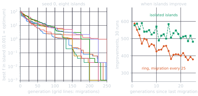
In the ring, a median of 0.240 [0.225, 0.247] of the search improvements fell in the first 5 generations after a migration. Isolated islands, binned by the same calendar, give 0.217 [0.206, 0.229], slightly above 0.2 because improvements become rarer as a run proceeds and the first generations of each interval come earlier. Pooled over all runs, the ring's improvements fell from 588 in the first generation after a migration to between 375 and 416 in the last ten, while the isolated islands' stayed between 482 and 590 throughout. Separately, 46% of migration events (median, [43%, 49%]) improved the receiving island's best value directly. The effect is real but modest in this setup: migrants arrive, sometimes better than anything the island has, and for a few generations afterward the island's own search finds improvements more often, which is what one would expect if crossover between newcomers and residents creates combinations neither held. The experiment does not test that mechanism directly.
A recurring difficulty in these comparisons is fairness. Holding the total population constant seems fair, but the quality a genetic algorithm reaches depends nonlinearly on population size, so a single population of 256 and 8 islands of 32 are not expected to reach the same quality in the same number of evaluations. Cantú-Paz (2000) argues that some reported superlinear speedups of parallel island models may have come from such comparisons, in particular from comparing an island model whose migration policy added selection pressure against a serial algorithm with the original, weaker pressure.
When islands help
Whitley, Rana, and Heckendorn (1999) asked whether island models do well on standard benchmarks partly because those benchmarks are separable, sums of terms that each depend on a few variables. Separate islands could solve different subproblems, and migration and crossover could then assemble the pieces. They compared a single population of 5,000 with islands of 50 to 1,000 members, using a steady-state genetic algorithm, on a deceptive function, on Rastrigin's function, and on two nonseparable functions. Islands helped on the deceptive function but not on Rastrigin's. A larger single population did not help on the deceptive function, where several populations converging to different solutions did; it helped a great deal on Rastrigin's function, where dividing the population only made it harder for good subsolutions to spread. On the nonseparable functions, the single large population performed best in the large-population experiments. With a smaller total population of 500 and mutation, island models with migration did as well as or better than the single population on all their test functions: on Rastrigin's function, 5 islands of 100 solved the problem in significantly fewer evaluations, and on Powell's function both island configurations found significantly better solutions. Their conclusion was that the separability hypothesis was only partly correct, and that island models are most likely to help where enlarging a single population does not.
Measured on Rastrigin's function and a deceptive function
The first part of island_model.py repeats a small version of that comparison. Both problems are encoded as bit strings, following Whitley, Rana, and Heckendorn. Rastrigin's function has 10 variables of 10 Gray-coded bits each (see binary encoding and Gray codes), and its minimum is 0. The deceptive function is theirs: 10 copies of a fully deceptive 4-bit subfunction in which 1111 scores 30 and 0000 scores 28, with the four bits of each copy spread across a 40-bit string, so that the maximum is 300 and a string of all zeros scores 280. Each island runs the same generational genetic algorithm: binary tournament selection, two-point crossover with probability 0.9, bit-flip mutation at rate $1/L$, and one elite. All configurations use 240 individuals for 250 generations, about 60,000 evaluations. The islands are 8 of 30, and each migration copies the best members of the source over the worst at the destination: 2 migrants per event in the ring and random topologies, and in the fully connected topology the best member of each of the other 7 islands. The table gives the median and interquartile range of the best value in the final population over 30 seeds, the number of runs that found the optimum, and the median gene diversity $H$ of the final population, the mean over loci of $2p(1 - p)$ where $p$ is the frequency of 1 across all 240 individuals ($H = 0$ means every locus is fixed).
| Configuration | Rastrigin: best (lower is better) | Optimum found | $H$ | Deceptive: best (higher is better) | $H$ |
|---|---|---|---|---|---|
| Panmictic | 0.24 [0.11, 1.19] | 0/30 | 0.179 | 282 [280, 282] | 0.168 |
| Isolated islands | 3.41 [3.00, 5.03] | 0/30 | 0.299 | 288 [286, 290] | 0.340 |
| Ring, $\tau = 1$ | 0.00 [0.00, 0.00] | 26/30 | 0.037 | 286 [284, 288] | 0.078 |
| Ring, $\tau = 5$ | 0.00 [0.00, 0.00] | 29/30 | 0.062 | 288 [286, 291.5] | 0.120 |
| Ring, $\tau = 25$ | 0.00 [0.00, 0.02] | 20/30 | 0.098 | 290 [288, 290] | 0.136 |
| Ring, $\tau = 100$ | 1.05 [0.06, 1.29] | 1/30 | 0.216 | 288 [286.5, 290] | 0.342 |
| Random, $\tau = 5$ | 0.00 [0.00, 0.00] | 26/30 | 0.068 | 288 [284.5, 290] | 0.117 |
| Random, $\tau = 25$ | 0.00 [0.00, 0.02] | 21/30 | 0.093 | 289 [288, 292] | 0.133 |
| Fully connected, $\tau = 1$ | 0.00 [0.00, 0.01] | 22/30 | 0.014 | 286 [284, 288] | 0.033 |
| Fully connected, $\tau = 25$ | 0.00 [0.00, 0.00] | 28/30 | 0.055 | 288 [286, 290] | 0.095 |
| Fully connected, $\tau = 100$ | 0.04 [0.02, 0.08] | 6/30 | 0.127 | 290 [288, 290] | 0.147 |
The script prints all four intervals for every topology; the rows omitted here follow the same pattern. No configuration found the deceptive function's optimum.
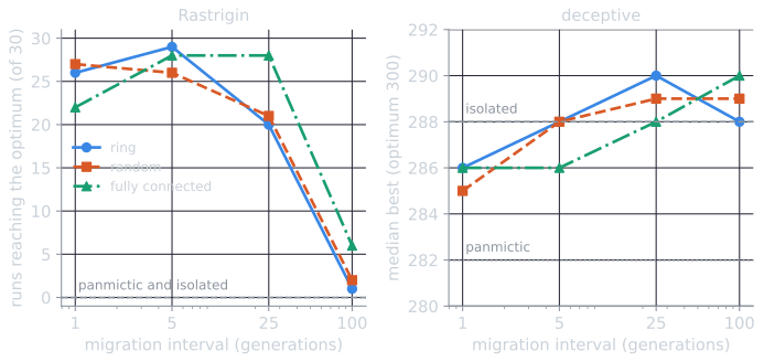
Several observations follow, all specific to this setup. On Rastrigin's function, every island model with migration at least every 25 generations beat the single population by a wide margin, and isolated islands did worst of all: 30 individuals were too few to solve the problem alone, and with no migration they never pooled what they found. Migration every 100 generations was too rare to help much in a ring, and helped somewhat more in the fully connected topology, which spreads a good individual to every island at once. On the deceptive function, every island configuration beat the single population, which was drawn to the deceptive attractor 0000 in nearly every subfunction: a score of 282, its median, is for example nine subfunctions at 0000 and one at 1111. Here isolation was not a handicap. Eight isolated islands, each settling on its own mixture of subfunction solutions, scored a median of 288, and migration every generation did worse, with medians of 285 to 286.
Diversity tells the same story from the other side. More frequent migration and denser topologies left less diversity at the end of the run: $H$ fell from 0.342 in the ring with $\tau = 100$ to 0.078 with $\tau = 1$ on the deceptive function, and to 0.033 in the fully connected topology with $\tau = 1$. The most reliable settings on Rastrigin's function were intermediate ones: migration every 5 generations in the ring (29 of 30 runs) and every 5 or 25 generations in the fully connected topology (28 of 30), against 26 and 22 runs with migration every generation. This agrees with the finding of Skolicki and De Jong (2005) that very frequent migration erodes the diversity that makes islands worth having, while very rare migration slows the search.
Following diversity through the run shows when the difference arises. island_dynamics.py reran five of the Rastrigin configurations recording $H$ and the best value every generation:
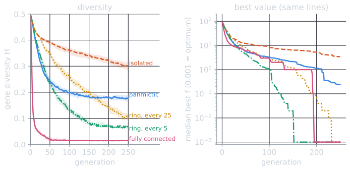
| Configuration | $H$ at generation 10 | $H$ at 50 | $H$ at 250 | Median best at 50 | Median best at 250 |
|---|---|---|---|---|---|
| Panmictic | 0.424 | 0.243 | 0.179 | 5.73 | 0.24 |
| Isolated | 0.445 | 0.390 | 0.299 | 12.16 | 3.41 |
| Ring, $\tau = 5$ | 0.431 | 0.232 | 0.062 | 4.44 | 0.00 |
| Ring, $\tau = 25$ | 0.445 | 0.350 | 0.098 | 8.19 | 0.00 |
| Fully connected, $\tau = 1$ | 0.088 | 0.022 | 0.014 | 5.99 | 0.00 |
Diversity alone does not explain success. The isolated islands keep the most diversity and do worst, because no island can use what the others find. The fully connected topology with $\tau = 1$ keeps the least and still reaches the optimum in 22 of 30 runs; one plausible reading is that its loci were fixed by the best of eight separate searches rather than by one, so less of what was fixed was wrong. What the successful configurations share is the combination: enough separation for the islands to find different partial solutions, and enough exchange for those solutions to meet. The direction of the Rastrigin result differs from Whitley, Rana, and Heckendorn's large-population experiment and agrees with their small-population one. With 240 individuals in total, the single population stalled near the optimum (median 0.24) without assembling it, which is the situation in which the extra diversity of islands can pay off.
Cellular evolutionary algorithms
A cellular evolutionary algorithm, also called a fine-grained or diffusion model, takes population structure to its limit. Each individual occupies a cell of a grid, usually a two-dimensional torus, and selection and mating are restricted to a small neighbourhood around it, such as the four nearest cells plus the cell itself (the von Neumann or "L5" neighbourhood) or the surrounding 3 × 3 block ("C9"). Each cell's offspring replaces it, often only if fitter. Neighbourhoods overlap, so there are no hard boundaries: good solutions spread across the grid gradually, while distant regions search different parts of the space. Alba and Dorronsoro (2008) give a book-length treatment, including a study of selection pressure in cellular genetic algorithms (ch. 4).
The cells can be updated synchronously, all at once from the previous grid, or asynchronously, one at a time in some order, so that a new individual can be selected by its neighbours in the same sweep.
Selection pressure in a cellular algorithm depends on the neighbourhood and the grid together. Sarma and De Jong (1996) analyzed the effect of neighbourhood size and shape on the selection pressure induced by local selection. Their analysis characterizes a neighbourhood by its radius, a measure of the spatial dispersion of its cells around its centre, rather than by its number of cells, and relates selection pressure to the ratio of the neighbourhood's radius to the grid's: configurations with similar ratios show similar takeover curves. Alba and Troya (2000) exploited this by changing the shape of the grid while keeping the neighbourhood fixed: a thin rectangular grid has a larger radius than a square one with the same number of cells, so its ratio is smaller and its selection pressure lower, which favours exploration.
The takeover experiment above shows the effect. With the L5 neighbourhood, 256 individuals on a $16 \times 16$ torus took a median of 22 generations to be taken over, three times as long as the panmictic population's 7; on a $4 \times 64$ torus, they took 61. In a square grid with a small neighbourhood, a good individual can spread only about one cell per generation in each direction, so takeover time grows with the grid's diameter rather than with the logarithm of the population size, as it does in a panmictic population. The thin grid's diameter is longer, and takeover is correspondingly slower. On a $16 \times 16$ torus the farthest cell is $8 + 8 = 16$ steps away; on a $4 \times 64$ torus it is $2 + 32 = 34$. A good individual does not advance one step every generation, because a cell adopts it only when one of its two tournament draws, out of five cells, lands on a neighbour that already holds it, so both takeover times exceed the diameters.
Choosing a model
Island and cellular models are both ways of slowing the spread of good solutions in exchange for diversity. Islands do it in coarse steps, with explicit parameters for how often and how much the subpopulations communicate; cellular models do it continuously, through the geometry of the grid. Both map naturally onto parallel hardware, islands onto separate processors or machines with infrequent messages, cellular models onto many fine-grained processors with constant local communication. Neither is better in general. They help most when a single population converges too early, which is a property of the problem, the population size and the selection scheme together. They can be combined, for instance as islands whose members are evaluated by a master and slaves, and island-style populations remain in use in recent systems: the program database of AlphaEvolve draws on them (Novikov and colleagues, 2025).
References
- Alba, E., and Dorronsoro, B. (2008). Cellular Genetic Algorithms. Operations Research/Computer Science Interfaces Series, vol. 42. Springer.
- Alba, E., and Tomassini, M. (2002). Parallelism and evolutionary algorithms. IEEE Transactions on Evolutionary Computation, 6(5), 443–462.
- Alba, E., and Troya, J. M. (2000). Cellular evolutionary algorithms: Evaluating the influence of ratio. In Parallel Problem Solving from Nature PPSN VI, Lecture Notes in Computer Science 1917, 29–38. Springer.
- Cantú-Paz, E. (1998). A survey of parallel genetic algorithms. Calculateurs Parallèles, Réseaux et Systèmes Répartis, 10(2), 141–171.
- Cantú-Paz, E. (2000). Efficient and Accurate Parallel Genetic Algorithms. Kluwer Academic Publishers.
- Cohoon, J. P., Hegde, S. U., Martin, W. N., and Richards, D. (1987). Punctuated equilibria: A parallel genetic algorithm. In Proceedings of the Second International Conference on Genetic Algorithms and Their Application, 148–154.
- Eiben, A. E., and Smith, J. E. (2015). Introduction to Evolutionary Computing, 2nd ed., chapter 5. Springer.
- Goldberg, D. E., and Deb, K. (1991). A comparative analysis of selection schemes used in genetic algorithms. In G. J. E. Rawlins (ed.), Foundations of Genetic Algorithms, 69–93. Morgan Kaufmann.
- Novikov, A., Vũ, N., Eisenberger, M., Dupont, E., Huang, P.-S., Wagner, A. Z., et al. (2025). AlphaEvolve: a coding agent for scientific and algorithmic discovery. arXiv:2506.13131.
- Sarma, J., and De Jong, K. (1996). An analysis of the effects of neighborhood size and shape on local selection algorithms. In Parallel Problem Solving from Nature PPSN IV, Lecture Notes in Computer Science 1141, 236–244. Springer.
- Skolicki, Z., and De Jong, K. (2005). The influence of migration sizes and intervals on island models. In Proceedings of the 7th Annual Conference on Genetic and Evolutionary Computation (GECCO 2005), 1295–1302.
- Tanese, R. (1989). Distributed genetic algorithms. In Proceedings of the Third International Conference on Genetic Algorithms, 434–439.
- Whitley, D., Rana, S., and Heckendorn, R. B. (1999). The island model genetic algorithm: On separability, population size and convergence. Journal of Computing and Information Technology, 7(1), 33–47.