Take four strings of five bits each, read each string as an unsigned integer $x$ between 0 and 31, and score it by $f(x) = x^2$. The best string, 11111, is obvious to a person, but suppose the scoring function were a black box. A genetic algorithm (GA) looks for good strings by imitating a population under natural selection: strings with higher scores get more copies in the next generation, the copies are paired and recombined by swapping pieces, and a few bits are flipped at random. Nothing in the procedure uses the formula $x^2$; it uses only the scores.
The version of this procedure that textbooks call the simple genetic algorithm (SGA), or the canonical GA, is the reference point for everything else in this topic. This article specifies it completely, works one generation of Goldberg's (1989, ch. 1) $x^2$ example by hand, follows a seeded run until it converges, and then measures where the algorithm falls short. The general evolutionary loop it instantiates is described in the evolutionary algorithm loop.
Where the SGA comes from
John Holland developed genetic algorithms at the University of Michigan as a model of adaptation, and his book (Holland, 1975) set out the framework: a population of fixed-length strings, reproduction in proportion to observed performance, and genetic operators, of which crossover was the principal one and mutation a background operator that restores lost bit values. Holland's student Kenneth De Jong (1975) tested such algorithms as function optimizers on a suite of test problems and measured how their behavior depended on population size, crossover rate and mutation rate. David Goldberg's (1989) textbook gave the algorithm the name used here and made it the standard first example. Whitley (1994) calls the same model the canonical genetic algorithm and notes that most of the existing theory of genetic algorithms applies solely or primarily to it, including the exact models of its dynamics developed in the early 1990s. Holland's schema theorem was also stated for this kind of algorithm.
Eiben and Smith (2015, ch. 6) summarize the SGA in five design choices:
| Component | Choice in the SGA |
|---|---|
| Representation | Bit strings of fixed length |
| Parent selection | Fitness-proportional, implemented by a roulette wheel |
| Recombination | One-point crossover, applied with probability $p_c$ |
| Mutation | Bit flip, each bit independently with probability $p_m$ |
| Survivor selection | Generational: the offspring replace the whole population |
The algorithm in full
The descriptions in the literature agree on these components but leave small details open, such as how parents are paired and how ties in the roulette wheel are broken. The specification below fixes every detail, so that a run is reproducible from its random seed. It is the one implemented in tools/experiments/evolution/sga.py in the site repository.
Representation and fitness. A candidate is a string of $L$ bits. The fitness function $f$ is to be maximized and must be non-negative, because selection probabilities are computed from it directly. A minimization problem, or one with negative values, must first be transformed, and the transformation matters, as the measurements below show.
Fitness-proportional selection. In a population of $N$ strings with fitnesses $f_1, \dots, f_N$, each selection event picks string $i$ with probability
$$p_i = \frac{f_i}{\sum_{j=1}^{N} f_j}.$$
The mating pool is filled by $N$ independent selections, so string $i$ receives on average $N p_i = f_i / \bar{f}$ copies, where $\bar{f}$ is the mean fitness. A string twice as fit as average expects two copies; a string at half the average expects half a copy. Whitley (1994) describes the selection step this way, as producing an intermediate population from which the next one is built. The roulette-wheel implementation draws a uniform number $r$ in $[0, \sum_j f_j)$ and picks the first string whose cumulative fitness exceeds $r$, which is the same as spinning a wheel whose slots are proportional to fitness.
Crossover. The pool is taken in the order of selection, and positions 1 and 2, 3 and 4, and so on form the pairs. Since the pool was filled by independent random draws, its order is already random. Each pair crosses with probability $p_c$. One-point crossover draws a site $k$ uniformly from $1, \dots, L - 1$ and exchanges the parts after bit $k$:
parents   1101|0      children  1101|1
          0110|1                0110|0
With probability $1 - p_c$, both parents pass to the next stage unchanged.
Mutation. Each bit of each child is flipped independently with probability $p_m$.
Replacement. The $N$ children form the next generation, and the parents are discarded. No individual survives from one generation to the next except as a copy made by selection.
In pseudocode:
SGA(f, L, N, pc, pm):
    P = N strings of L random bits
    repeat until the termination condition holds:
        evaluate f on every string in P
        pool = N strings drawn from P, each with probability f_i / sum(f)
        Q = empty
        for j = 1, 3, 5, ..., N - 1:
            a, b = copies of pool[j], pool[j + 1]
            with probability pc:
                k = uniform integer in 1 .. L - 1
                swap the bits of a and b after position k
            flip each bit of a and of b with probability pm
            add a and b to Q
        P = Q
The termination condition is usually a fixed number of generations, since the algorithm cannot recognize an optimum. Because the best string of one generation can disappear in the next, an implementation should record the best string ever evaluated separately from the population.
One generation by hand
Goldberg (1989, ch. 1) works this example through by hand. The initial population of four strings has total fitness 1,170 and mean 292.5:
| String | $x$ | $f(x) = x^2$ | $p_i = f_i / \sum f$ | Expected copies $f_i / \bar{f}$ |
|---|---|---|---|---|
| 01101 | 13 | 169 | 0.1444 | 0.578 |
| 11000 | 24 | 576 | 0.4923 | 1.969 |
| 01000 | 8 | 64 | 0.0547 | 0.219 |
| 10011 | 19 | 361 | 0.3085 | 1.234 |
Spinning the wheel. Laying the four fitness values end to end gives each string an interval of the number line from 0 to the total fitness, 1,170:
| String | Interval of $r$ | Width |
|---|---|---|
| 1: 01101 | $[0, 169)$ | 169 |
| 2: 11000 | $[169, 745)$ | 576 |
| 3: 01000 | $[745, 809)$ | 64 |
| 4: 10011 | $[809, 1170)$ | 361 |
A spin draws $u$ uniformly from $[0, 1)$, sets $r = 1170\,u$, and selects the string whose interval contains $r$. Four spins with $u = 0.10, 0.35, 0.55$ and $0.85$, for example, give $r = 117.0, 409.5, 643.5$ and $994.5$, which select strings 1, 2, 2 and 4. Bending the number line into a circle gives the wheel.
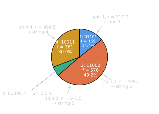
Suppose the four spins of the wheel select strings 1, 2, 2 and 4, as in the example, so the pool is 01101, 11000, 11000, 10011. String 2 receives two copies, close to its expected 1.97; string 3, with an expectation of 0.22, receives none.
The expected copies are only averages. Since the four spins are independent, the number of copies string $i$ receives is binomial, with 4 trials and success probability $p_i$:
| String | $p_i$ | 0 copies | 1 | 2 | 3 | 4 |
|---|---|---|---|---|---|---|
| 1: 01101 | 0.1444 | 0.536 | 0.362 | 0.092 | 0.010 | 0.000 |
| 2: 11000 | 0.4923 | 0.066 | 0.258 | 0.375 | 0.242 | 0.059 |
| 3: 01000 | 0.0547 | 0.799 | 0.185 | 0.016 | 0.001 | 0.000 |
| 4: 10011 | 0.3085 | 0.229 | 0.408 | 0.273 | 0.081 | 0.009 |
(Probabilities rounded to three places; entries shown as 0.000 are below 0.0005.) The best string, 11000, is lost altogether in 6.6 percent of generations, and in another 25.8 percent it receives only one copy although it expects nearly two. The pool used here, one copy of string 1, two of string 2 and one of string 4 in any order, has probability $\binom{4}{1}\binom{3}{2}\, p_1\, p_2^2\, p_4 = 12 \times 0.1444 \times 0.4923^2 \times 0.3085 = 0.130$. This sampling noise, separate from selection itself, is what stochastic universal sampling was designed to reduce.
Crossover. The first pair, 01101 and 11000, crosses at site 4. The second pair, 11000 and 10011, crosses at site 2:
| Pair | Site | Children | $x$ | $f(x)$ |
|---|---|---|---|---|
| 0110|1 and 1100|0 | 4 | 01100, 11001 | 12, 25 | 144, 625 |
| 11|000 and 10|011 | 2 | 11011, 10000 | 27, 16 | 729, 256 |
Bit by bit, the first child takes positions 1 to 4 of its first parent and position 5 of its second: 0110 from 01101 and 0 from 11000, giving 01100. The second child takes the complementary pieces, 1100 from 11000 and 1 from 01101, giving 11001. A cut at site $k$ always produces two children that between them hold exactly the bits of the two parents, position by position.
Mutation. With $p_m = 0.001$ and 20 bits in the population, the expected number of flips is $20 \times 0.001 = 0.02$, and the probability that no bit flips is $0.999^{20} = 0.980$, so mutation leaves all four children alone.
The result. In one generation the total fitness has risen from 1,170 to 1,754, the mean from 292.5 to 438.5, and the maximum from 576 to 729. Two of the children, 11001 and 11011, are better than any parent. Crossover combined the leading 11 of 11000 with the trailing ones of 01101 and 10011, which no single parent had together. The schema theorem article follows three patterns of bits, such as "first bit 1", through this same generation and compares their counts with what the theorem predicts.
The demo below runs the same algorithm. It starts from Goldberg's four strings, so its first table repeats the selection probabilities above; each press of Step spins the wheel four times, crosses the pairs and mutates the children, showing the cut sites and any flipped bits. Its random numbers come from its own seeded generator, so its runs differ from the Python script's.
A seeded run
The same problem run to completion shows the other side of the algorithm. With $N = 4$, $p_c = 1.0$, $p_m = 0.001$ and seed 1, the script prints this run:
| Generation | Population (fitness) | Mean |
|---|---|---|
| 0 | 00101 (25), 11100 (784), 10110 (484), 11001 (625) | 479.5 |
| 1 | 11100 (784), 11100 (784), 11001 (625), 10110 (484) | 669.2 |
| 2 | 10110 (484), 11100 (784), 10110 (484), 11100 (784) | 634.0 |
| 3 | 10100 (400), 11110 (900), 10110 (484), 10110 (484) | 567.0 |
| 6 | 11110 (900), 11110 (900), 11110 (900), 11110 (900) | 900.0 |
In generation 1 the only string ending in 1 is 11001. Its selection probability is $625 / 2677 = 0.233$, so the chance that four spins all miss it is $(1 - 0.233)^4 = 0.345$, and in this run they did. From generation 2 onward no string has a 1 in the last position. Crossover cannot create a bit value that no parent carries, so the optimum 11111 can now be reached only by mutation. In generation 3 crossover of 10110 and 11100 at site 2 produced 11110 ($x = 30$), and by generation 6 every string was a copy of it. The run then stayed at 900 until the twentieth generation. The only mutation in that time came in generation 18, when a flip of the first bit produced 01110 (196), which selection removed in the next generation. With $p_m = 0.001$, the chance that a given bit position is flipped in at least one of four strings in a generation is about 0.004.
This is premature convergence: the population has lost the diversity it needs before reaching the optimum. A population of four is unrealistically small, but it shows the mechanism clearly. Over 30 seeds (0 to 29) with 50 generations, the $N = 4$ algorithm found 11111 in 9 runs. With $N = 20$ it found it in 29 runs, but this says little: each random 5-bit string is 11111 with probability $1/32$, so a population of 20 contains the optimum from the start in almost half of all runs. Problems where a GA earns its keep are much larger than this one. The causes and remedies of premature convergence are the subject of selection pressure and premature convergence.
Classic parameter settings
The SGA has three numerical parameters, $N$, $p_c$ and $p_m$, and early work spent considerable effort on choosing them.
- De Jong (1975) studied them on his five test functions. Mills, Filliben and Haines (2015), reviewing this work, report that his best results came from a population of 50, single-point crossover with probability 0.6, a mutation probability of 0.001 per bit, and a variant in which the best individual always survived.
- Grefenstette (1986) treated the choice as an optimization problem in its own right and searched the space of GA parameters with a meta-level GA, on De Jong's functions. The best setting he found for online performance (the average of all evaluations so far) used a population of 30, crossover probability 0.95, mutation probability 0.01, and the elitist strategy; for offline performance (the average of the best values so far) the best setting used a population of 80, crossover probability 0.45 and mutation probability 0.01, without elitism. Mutation rates above 0.05 were generally harmful, and so was no mutation at all.
- Schaffer, Caruana, Eshelman and Das (1989) ran a large factorial experiment on a wider set of functions and found interactions between the three parameters: small populations were sensitive to the mutation rate and much less to the crossover rate. The settings usually quoted from their study are a population of 20 to 30, crossover probability 0.75 to 0.95 and mutation probability 0.005 to 0.01.
These settings are still quoted as defaults, but they were found for particular test functions, particular performance measures and particular variants of the algorithm, and they disagree with one another. Grefenstette's two best settings differ by a factor of two in crossover rate because they optimize different measures. Mills, Filliben and Haines (2015) summarize the later literature as having reached no general agreement. Eiben and Smith (2015, ch. 7) treat parameter tuning as a problem to be solved for each application, with its own methods, rather than one with a universal answer. A common modern default for mutation, one flip per string on average ($p_m = 1/L$), is close to Schaffer and colleagues' range for strings of about 100 to 200 bits.
What the SGA does well and badly
The SGA's strengths come from its simplicity. It needs only a way to encode candidates as bit strings and a fitness value for each, and every component is easy to implement and to analyze. It is the algorithm for which genetic algorithm theory is most developed, and it remains a reference against which variants are compared.
Its weaknesses come from two of its choices: fitness-proportional selection and full generational replacement. The script measures them on OneMax with $L = 100$ (fitness is the number of ones), $N = 50$, $p_c = 0.6$ and 200 generations, 30 seeds for each setting. The table reports medians, with the interquartile range in brackets.
| $p_m$ | Fitness used | Elitism | Best ever | Best in final population | Runs that lost their best |
|---|---|---|---|---|---|
| 0.001 | ones | no | 74 [72, 75] | 72 [71, 74] | 25 of 30 |
| 0.001 | ones | yes | 87 [85, 88.75] | 87 [85, 88.75] | 0 |
| 0.001 | ones + 100 | no | 67 [65, 68] | 61 [59, 64] | 29 of 30 |
| 0.01 | ones | no | 76 [75, 77] | 70 [67, 71] | 30 of 30 |
| 0.01 | ones | yes | 89.5 [88, 91.75] | 89.5 [88, 91.75] | 0 |
| 0.01 | ones + 100 | no | 71 [70, 72] | 63.5 [61, 65] | 28 of 30 |
Three weaknesses show in these numbers, and the figure follows the $p_m = 0.01$ runs generation by generation.
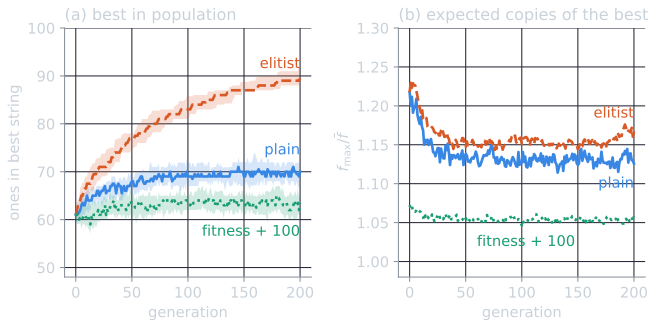
Selection pressure fades. Fitness-proportional selection gives the best string $f_{\max} / \bar{f}$ expected copies. Early in a run, fitness values differ a lot and the best strings multiply quickly. Later, when the population's fitness values lie close together, the ratio is close to 1: in the final generation of the runs without elitism, its median was 1.05 for $p_m = 0.001$ and 1.13 for $p_m = 0.01$. On OneMax the ratio has a simple reading. In the final generation of a typical plain run, the best string has about 70 ones and the population mean is about 62, so the best expects $70/62 \approx 1.13$ copies, only slightly more than an average string. Mutation pulls the other way: a string with $k$ ones loses on average $p_m k$ ones and gains $p_m (L - k)$, a net change of $0.01 \times (38 - 62) = -0.24$ ones per generation for a string at the mean. Selection that barely favours the best string can only just offset that loss, and the population stalls where the two balance. Selection then barely distinguishes good strings from average ones, and after 10,000 evaluations no run without elitism had found a string with more than 82 ones. Eiben and Smith (2015, ch. 5) describe this loss of selection pressure as a known drawback of fitness-proportional selection.
Results depend on how fitness is expressed. Adding 100 to every fitness value changes no comparison between strings, but it shrinks the ratio $f_{\max} / \bar{f}$ further (a median of 1.02 for $p_m = 0.001$), and the median best-ever result fell from 74 to 67. The algorithm is not invariant to translating the fitness function, so the choice of transformation for a minimization problem, such as $1/(1 + f)$, quietly sets the selection pressure. Rank-based and tournament selection depend only on the order of fitness values, which removes this problem.
The best string is lost. With generational replacement, the best string survives only if selection copies it and crossover and mutation leave it intact. In 25 to 30 of every 30 runs without elitism, the final population was worse than the best string seen earlier. Keeping the best string, the elitist variant used by De Jong and by Grefenstette's online setting, raised the median final result from 72 to 87 for $p_m = 0.001$. It has a cost in other settings: an elite that is never displaced can pull the whole population toward a local optimum.
The SGA was also slow on this problem. A population of 50 run for 200 generations spends 10,000 evaluations, and even with elitism no run reached the optimum of 100; the best reached 95. OneMax is easy for simpler methods, as the measurements in the evolutionary algorithm loop show for a single-string $(1+1)$ evolutionary algorithm. The SGA's population, crossover and weak selection buy robustness on rugged problems, not speed on smooth ones. Its bit-string representation adds a further weakness when the variables are real numbers, discussed in binary encoding and Gray codes.
Later variants
Most later genetic algorithms change one SGA component at a time, and each change answers one of the problems above.
- Elitism copies the best one or few individuals into the next generation unchanged, so the best fitness in the population never decreases.
- Rank-based and tournament selection replace fitness-proportional selection, making selection pressure independent of the scale and offset of the fitness function. Stochastic universal sampling keeps fitness-proportional selection but places $N$ equally spaced pointers around the wheel and spins once, so that the number of copies each string receives follows its expected value more closely (Whitley, 1994): a string expecting 1.36 copies receives one or two, never zero or three. These methods are compared in selection pressure and premature convergence.
- Steady-state GAs replace a few individuals at a time instead of the whole population. De Jong (1975) already parameterized replacement by a generation gap, the fraction of the population replaced each generation, which is 1 in the SGA; Grefenstette's meta-GA searched over it as well. Whitley's GENITOR (Whitley, 1989) produced one offspring at a time, used rank-based selection, and inserted each offspring in place of the worst member of the population. Eiben and Smith (2015, ch. 5) present generational and steady-state models as the two ends of this range.
- Other operators and representations. Two-point and uniform crossover, and real-valued, permutation and tree representations with their own operators, are covered in crossover and mutation operators and binary encoding and Gray codes.
The course's own binary GA, which combined the SGA's roulette wheel with two-point crossover and generational replacement on De Jong's functions, is examined in a binary GA on De Jong's test functions, with results over 30 seeds.
References
- De Jong, K. A. (1975). An Analysis of the Behavior of a Class of Genetic Adaptive Systems. PhD dissertation, University of Michigan.
- Eiben, A. E., and Smith, J. E. (2015). Introduction to Evolutionary Computing, 2nd ed., chapters 5, 6 and 7. Springer.
- Goldberg, D. E. (1989). Genetic Algorithms in Search, Optimization, and Machine Learning, chapter 1. Addison-Wesley.
- Grefenstette, J. J. (1986). Optimization of control parameters for genetic algorithms. IEEE Transactions on Systems, Man, and Cybernetics, 16(1), 122–128.
- Holland, J. H. (1975). Adaptation in Natural and Artificial Systems. University of Michigan Press.
- Mills, K. L., Filliben, J. J., and Haines, A. L. (2015). Determining relative importance and effective settings for genetic algorithm control parameters. Evolutionary Computation, 23(2), 309–342.
- Schaffer, J. D., Caruana, R. A., Eshelman, L. J., and Das, R. (1989). A study of control parameters affecting online performance of genetic algorithms for function optimization. In Proceedings of the Third International Conference on Genetic Algorithms, 51–60. Morgan Kaufmann.
- Whitley, D. (1989). The GENITOR algorithm and selection pressure: Why rank-based allocation of reproductive trials is best. In Proceedings of the Third International Conference on Genetic Algorithms, 116–121. Morgan Kaufmann.
- Whitley, D. (1994). A genetic algorithm tutorial. Statistics and Computing, 4(2), 65–85.