Minimize $f(\mathbf{x}) = \sum_i x_i^2$ in ten dimensions, starting from a random point in $[-2, 2]^{10}$. Add a small Gaussian perturbation with standard deviation $\sigma = 0.01$ to every coordinate, keep the new point if it is no worse, and repeat. In 30 seeded runs the median value of $f$ fell from about 16 to $10^{-2.1}$ in 1,000 evaluations, reached $10^{-3.7}$ after 2,000, and then stopped moving: after 3,000 evaluations it was $10^{-3.8}$. With $\sigma = 1.2$, the value fell from 16 to about 1.6 and stalled there. Now let $\sigma$ grow by a factor $e^{1/3}$ after every success and shrink by $e^{-1/12}$ after every failure. The same runs reached $f \le 10^{-8}$ after a median of 664 evaluations and $10^{-40}$ after 3,000, falling by the same number of decimal places in every stretch of 1,000 evaluations.
The algorithm is the (1+1) evolution strategy, and the step-size rule is a form of Rechenberg's 1/5 success rule. This article explains why a fixed step size must stall, where the number 1/5 comes from, how the rule is implemented, and what it cannot do. It assumes the general loop of an evolutionary algorithm and builds on hill climbing, of which the (1+1)-ES is the continuous, randomized form. Population-based strategies and step sizes that evolve with the individuals are the subject of $(\mu,\lambda)$ selection and self-adaptation.
The (1+1)-ES
The strategy keeps one parent $\mathbf{x} \in \mathbb{R}^n$ and one step size $\sigma > 0$. Each generation:
- Draw $\mathbf{z} \sim \mathcal{N}(\mathbf{0}, \mathbf{I})$, a vector of $n$ independent standard normal numbers.
- Form the offspring $\mathbf{y} = \mathbf{x} + \sigma \mathbf{z}$ and evaluate $f(\mathbf{y})$.
- If $f(\mathbf{y}) \le f(\mathbf{x})$, the generation is a success and $\mathbf{y}$ replaces $\mathbf{x}$. Otherwise $\mathbf{y}$ is discarded.
- Update $\sigma$ by a step-size rule, or leave it unchanged.
The name follows the notation of Beyer and Schwefel (2002, §3.1): one parent, one offspring, and "+" for selection among parent and offspring together, so the best point found is never lost. The mutation is isotropic: every direction is equally likely, and the surfaces of constant density are spheres around the parent. Its only parameter is $\sigma$, the standard deviation of each coordinate's change, often called the mutation strength. The expected length of a step is close to $\sigma\sqrt{n}$.
This is the strategy that Rechenberg and Schwefel used in their flow experiments in Berlin in the 1960s, such as a jointed plate in a wind tunnel. Those experiments changed the variables in discrete steps; Gaussian mutations came after a simulation study showed that discrete steps could leave the search stuck (history of evolutionary computation; Beyer and Schwefel, 2002, §2). As a search algorithm it is a first-choice hill climber whose neighborhood is all of $\mathbb{R}^n$, weighted toward nearby points. Its behavior is governed almost entirely by $\sigma$.
Why a fixed step size stalls
The sphere $f(\mathbf{x}) = \lVert \mathbf{x} \rVert^2$ makes the problem clear. Let $R = \lVert \mathbf{x} \rVert$ be the parent's distance to the optimum. A success is an offspring inside the ball of radius $R$.
- If $\sigma$ is very small compared with $R/n$, the surface of the ball looks flat from the parent's position, and almost exactly half of all mutations land on the improving side. The success probability approaches 1/2, but each success moves the parent only a distance of order $\sigma$, so progress is slow.
- If $\sigma$ is large compared with $R/n$, nearly every mutation overshoots the ball. Successes become rare, and progress is slow again.
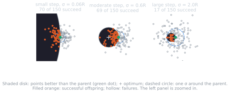
Between the two lies a band of step sizes with useful progress, which Rechenberg (1973) called the evolution window (Beyer and Schwefel, 2002, §4.1.1). The difficulty is that the window moves. As the parent approaches the optimum, $R$ shrinks, and a step size that was well placed becomes too large. The run with $\sigma = 0.01$ in the introduction did well while $R$ was large, then stopped near $f = 10^{-3.8}$, where $R \approx 0.013$ and $\sigma n / R \approx 8$. There, the asymptotic formula given below puts the success probability at about $4 \times 10^{-5}$, so a success takes tens of thousands of evaluations on average. Beyer and Schwefel (2002, §4.1.1) show the same effect, and note that the strategy with constant $\sigma$ is still globally convergent in principle (Rechenberg, 1973). Convergence in the limit is of no practical use if each further digit of accuracy costs ten times more than the last.
Rechenberg's progress-rate analysis
Rechenberg's dissertation, completed in 1971 and published as a book in 1973, analyzed the (1+1)-ES with Gaussian mutations on two model functions, the sphere and a corridor: a linear function to be optimized inside a band bounded by $2(n-1)$ inequality constraints (Beyer and Schwefel, 2002, §2.2 and §4.1.2). The measure was the progress rate $\varphi$, the expected distance traveled toward the optimum in one generation. Beyer and Schwefel summarize his results in three points: the progress rate is inversely proportional to the number of variables; linear convergence order can be reached if the mutation strength is kept permanently at the right order of magnitude; and the optimal mutation strength corresponds to a success probability that does not depend on $n$ and is roughly one fifth for both models.
The sphere
On the sphere, the natural quantities are normalized by $R$ and $n$. Write $\sigma^* = \sigma n / R$ for the normalized mutation strength and $\varphi^* = \varphi n / R$ for the normalized progress rate, where $\varphi = \mathrm{E}[R - R']$ is the expected decrease of the distance in one generation, with $R' = R$ when the offspring is rejected. In the limit $n \to \infty$ they are related by a single curve (Beyer and Schwefel, 2002, §4.1.2, Fig. 10, after Rechenberg, 1973):
$$\varphi^*(\sigma^*) = \frac{\sigma^*}{\sqrt{2\pi}} \, e^{-\sigma^{*2}/8} \;-\; \frac{\sigma^{*2}}{2} \left( 1 - \Phi\!\left(\frac{\sigma^*}{2}\right) \right), \qquad P_s(\sigma^*) = 1 - \Phi\!\left(\frac{\sigma^*}{2}\right),$$
where $\Phi$ is the standard normal distribution function and $P_s$ the success probability. Both formulas follow from a short calculation, which shows where the normalization comes from.
Deriving the curve
Put the optimum at the origin and the parent $\mathbf{x}$ at distance $R$. Split the mutation vector $\mathbf{z}$ into its component toward the optimum, $z_1 = -\mathbf{x}^\top\mathbf{z}/R$, which is standard normal, and the $n - 1$ components perpendicular to it.
- Expand the offspring's squared distance. With $\mathbf{y} = \mathbf{x} + \sigma\mathbf{z}$, $$\lVert \mathbf{y} \rVert^2 = R^2 + 2\sigma\,\mathbf{x}^\top\mathbf{z} + \sigma^2 \lVert \mathbf{z} \rVert^2 = R^2 - 2\sigma R\, z_1 + \sigma^2 \lVert \mathbf{z} \rVert^2.$$ The middle term is the gain from moving toward the optimum; it is linear in $\sigma$ and has a random sign. The last term is the cost of the step's length, which is quadratic in $\sigma$ and always positive.
- Replace $\lVert \mathbf{z} \rVert^2$ by $n$. It is a sum of $n$ squared standard normals, with mean $n$ and standard deviation $\sqrt{2n}$, so its relative fluctuation vanishes as $n$ grows. The cost term becomes $\sigma^2 n$: almost all of a random step is sideways.
- Find the natural scale. The gain $2\sigma R z_1$ and the cost $\sigma^2 n$ are of the same size when $\sigma$ is of order $R/n$. That is why the step size is measured as $\sigma^* = \sigma n / R$. Multiplying the improvement $R^2 - \lVert \mathbf{y} \rVert^2$ by $n / (2R^2)$ gives the normalized improvement $$Q = \frac{n\,(R^2 - \lVert \mathbf{y} \rVert^2)}{2R^2} \approx \sigma^* z_1 - \frac{\sigma^{*2}}{2},$$ a normal random variable with mean $-\sigma^{*2}/2$ and standard deviation $\sigma^*$.
- Success probability. The offspring is accepted when $Q > 0$, that is when $z_1 > \sigma^*/2$, which happens with probability $P_s = 1 - \Phi(\sigma^*/2)$.
- Progress. The new distance is $R' = R\sqrt{1 - 2Q/n} \approx R(1 - Q/n)$ for large $n$, so an accepted offspring moves the parent $R - R' \approx RQ/n$ closer, and a rejected one moves it not at all. Hence $\varphi^* = n\,\mathrm{E}[R - R']/R \approx \mathrm{E}[Q\, \mathbb{1}(Q > 0)]$.
- Evaluate the expectation. With $a = \sigma^*/2$ and $\phi$ the standard normal density, $\mathrm{E}[z_1 \mathbb{1}(z_1 > a)] = \phi(a)$ and $P(z_1 > a) = 1 - \Phi(a)$, so $$\varphi^* = \sigma^* \phi\!\left(\tfrac{\sigma^*}{2}\right) - \frac{\sigma^{*2}}{2}\left(1 - \Phi\!\left(\tfrac{\sigma^*}{2}\right)\right),$$ which is the formula above, since $\phi(\sigma^*/2) = e^{-\sigma^{*2}/8}/\sqrt{2\pi}$.
The approximation that matters most is the one in step 2, and it can be checked directly. The script tools/experiments/evolution/one_fifth_worked.py drew 200,000 mutations at $\sigma^* = 1.224$ from a parent at distance 1 and computed $Q$ exactly. The model predicts a mean of $-0.749$, a standard deviation of $1.224$, and $P(Q > 0) = 0.270$. For $n = 1000$ the sample gave $-0.751$, $1.228$ and $0.271$; for $n = 100$, $-0.749$, $1.225$ and $0.272$; for $n = 10$, $-0.747$, $1.269$ and $0.290$. In ten dimensions the spread of $\lVert \mathbf{z} \rVert^2$ is still large enough to widen $Q$ and lift the success probability by two points.
The curve gives these values:
| $\sigma^*$ | 0.5 | 1.0 | 1.224 | 2.0 | 3.0 | 4.0 |
|---|---|---|---|---|---|---|
| $\varphi^*$ | 0.143 | 0.198 | 0.202 | 0.167 | 0.088 | 0.034 |
| $P_s$ | 0.401 | 0.309 | 0.270 | 0.159 | 0.067 | 0.023 |
The maximum progress, $\varphi^* \approx 0.202$, is reached at $\sigma^* \approx 1.224$, where the success probability is about 0.27. Beyer and Schwefel (2002, §4.1.2) give the same optimal success probability, $\hat{P}_s \approx 0.27$. To check the asymptotic formula at the dimensions used below, the experiment script drew 200,000 mutations at $\sigma^* = 1.224$ from a parent at distance 1. The estimates were $\varphi^* = 0.214$ and $P_s = 0.290$ for $n = 10$, $0.208$ and $0.277$ for $n = 30$, and $0.203$ and $0.272$ for $n = 100$, approaching the limit as $n$ grows.
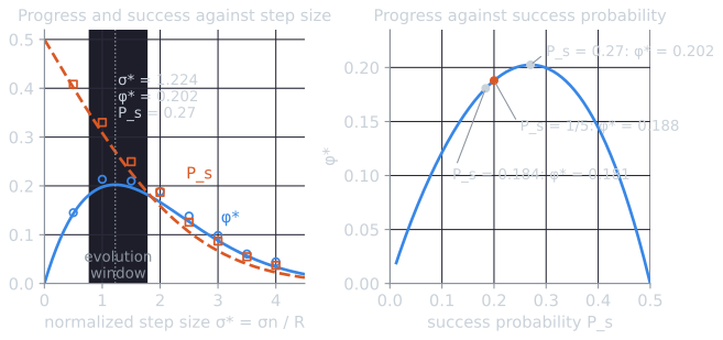
The right-hand panel answers a question the table raises: if 0.27 is optimal on the sphere, how much does aiming at 0.2 cost? Eliminating $\sigma^*$ through $\sigma^* = 2\Phi^{-1}(1 - P_s)$ gives $\varphi^*$ as a function of $P_s$ alone. At $P_s = 0.2$, $\sigma^* = 1.683$ and $\varphi^* = 0.188$, 92.8% of the maximum; at the corridor's 0.184, $\varphi^* = 0.181$, 89.3%. Any success probability between 0.187 and 0.349 keeps at least 90% of the best progress. The rule's target does not have to be exact. What it has to do is keep $\sigma^*$ inside the window as $R$ changes by many orders of magnitude, and that is what a fixed $\sigma$ cannot do.
Two consequences follow from the normalization. The progress per generation is $\varphi = \varphi^* R / n$: it is proportional to the remaining distance, so the distance shrinks by a constant factor per generation, and it is inversely proportional to $n$. Both are among the results Beyer and Schwefel attribute to Rechenberg.
The corridor and the compromise
On the corridor, the optimal success probability is about 0.184 (Rechenberg, 1973, p. 122, as cited by Beyer and Schwefel, 2002, §4.1.2). Auger and Hansen (2016, app. A) give the asymptotic value as $1/(2e) \approx 0.184$. Two very different model functions thus gave optimal success probabilities of 0.27 and 0.18. Both models were regarded as typical of real objective functions, and Rechenberg proposed the compromise of 0.2, which became the 1/5 success rule (Beyer and Schwefel, 2002, §4.1.2):
To obtain nearly optimal local performance of the (1+1)-ES, tune the mutation strength so that the measured success rate is about 1/5. If the success rate is below 1/5, decrease $\sigma$; if it is above, increase $\sigma$.
The rule needs no knowledge of $R$ or of the optimum. It works because $P_s$ falls monotonically as $\sigma^*$ grows, so the observed success rate tells the algorithm on which side of the target it is. Auger and Hansen (2016) note that essentially the same algorithm was also introduced, under the name adaptive step size random search, by Schumer and Steiglitz (1968).
Implementations
Rechenberg and Schwefel's version estimates the success probability over a block of generations (Beyer and Schwefel, 2002, §4.1.2, Fig. 11):
- Run the (1+1)-ES for $G$ generations with $\sigma$ fixed, counting the successes $G_s$.
- Estimate $P_s = G_s / G$.
- Set $\sigma \leftarrow \sigma / a$ if $P_s > 1/5$, $\sigma \leftarrow \sigma a$ if $P_s < 1/5$, and leave $\sigma$ unchanged if $P_s = 1/5$.
- Repeat.
The factor $a < 1$ depends on the function, on $n$, and on $G$. For $n \ge 30$, $G = n$ is a reasonable choice, and Schwefel (1975) recommended $0.85 \le a < 1$. Eiben and Smith (2015, §8.2.1) give the wider range $0.817 \le a \le 1$. On our reading, 0.817 is $e^{-0.202}$: on the sphere at the best possible progress rate, $R$ shrinks by a factor $e^{-\varphi^*} \approx 0.817$ every $n$ generations, and $\sigma$ must shrink at the same rate to keep $\sigma^*$ constant. A smaller decrease per block caps the convergence rate, as the experiment below shows.
The per-generation version updates $\sigma$ after every evaluation. With target success probability $p_{\text{target}}$ and a learning rate $\alpha > 0$, Auger and Hansen (2016, eq. A.11) write it as
$$\sigma \leftarrow \sigma \exp\!\left( \alpha \, \frac{\mathbb{1}[\text{success}] - p_{\text{target}}}{1 - p_{\text{target}}} \right).$$
With $p_{\text{target}} = 1/5$ and $\alpha = 1/3$, the values used in their simulations, a success multiplies $\sigma$ by $e^{1/3} \approx 1.40$ and a failure by $e^{-1/12} \approx 0.92$. Four failures undo one success, so $\sigma$ is stationary on average exactly when one generation in five succeeds. Glasmachers (2020) attributes this variant of the (1+1)-ES to Kern et al. (2004) and analyzes the general form, with separate constants for success and failure. Auger and Hansen also point out that a converging run settles below the target: $\sigma$ must keep shrinking as the parent approaches the optimum, which requires slightly more failures than the target allows, so the success rate actually achieved is somewhat less than 1/5.
The per-generation rule, generation by generation
The first generations of one run show the rule finding the window. Seed 0 of the sphere experiment below, $n = 10$, starts at $f = 16.6391$, so $R = 4.0791$, with $\sigma = 1.2$ and hence $\sigma^* = 1.2 \times 10 / 4.0791 = 2.942$, well above the window. The table lists the step size used in each generation, the offspring's value, the outcome, and the step size and normalized step size after the update (values rounded to four and three decimals; from one_fifth_worked.py):
| Generation | $\sigma$ used | $f(\mathbf{y})$ | Outcome | $\sigma$ after | $\sigma^*$ after |
|---|---|---|---|---|---|
| 1 | 1.2000 | 37.4157 | failure | 1.1041 | 2.707 |
| 2 | 1.1041 | 21.8605 | failure | 1.0158 | 2.490 |
| 3 | 1.0158 | 25.8605 | failure | 0.9346 | 2.291 |
| 4 | 0.9346 | 29.5501 | failure | 0.8598 | 2.108 |
| ... | 7 more failures | ||||
| 12 | 0.4798 | 16.9879 | failure | 0.4415 | 1.082 |
| 13 | 0.4415 | 20.3930 | failure | 0.4062 | 0.996 |
| 14 | 0.4062 | 16.8662 | failure | 0.3737 | 0.916 |
| 15 | 0.3737 | 14.7445 | success | 0.5215 | 1.358 |
| 16 | 0.5215 | 20.9675 | failure | 0.4798 | 1.250 |
| ... | 5 more failures | ||||
| 22 | 0.3163 | 17.1113 | failure | 0.2910 | 0.758 |
| 23 | 0.2910 | 11.1470 | success | 0.4062 | 1.217 |
| 24 | 0.4062 | 15.9300 | failure | 0.3737 | 1.119 |
Each failure multiplies $\sigma$ by $e^{-1/12} = 0.9200$ and each success by $e^{1/3} = 1.3956$. Fourteen failures in a row brought $\sigma^*$ from 2.94 down into the evolution window, which on the figure above runs from 0.78 to 1.78, and on to 0.92; the first success, at generation 15, then raised it to 1.36, partly because $\sigma$ grew and partly because $R$ shrank. After 24 generations, with 2 successes and 22 failures, $\sigma = 1.2\, e^{2/3 - 22/12} = 0.3737$, which depends only on the counts, not their order. The rule never needs to know $R$. It sees only the stream of successes and failures, and the step size follows from them.
Experiment: the sphere
Script: tools/experiments/evolution/one_plus_one_es.py. Each of 30 runs (seeds 0 to 29) starts from a point drawn uniformly from $[-2, 2]^n$ with $\sigma_0 = 1.2$, and has a budget of $300n$ evaluations. Six step-size rules were compared: two fixed values of $\sigma$; an "oracle" that sets $\sigma = 1.224 R/n$ before every mutation using the known optimum; the block rule with $G = n$ and $a = 0.85$ or $a = 0.817$; and the per-generation rule with $\alpha = 1/3$. Medians over 30 runs, with interquartile ranges in parentheses:
| Rule | Evaluations to $f \le 10^{-8}$, $n = 10$ | Normalized rate, $n = 10$ | Success rate, $n = 10$ | Evaluations to $f \le 10^{-8}$, $n = 30$ | Normalized rate, $n = 30$ | Success rate, $n = 30$ |
|---|---|---|---|---|---|---|
| Fixed $\sigma = 1.2$ | not reached | not reached | ||||
| Fixed $\sigma = 0.01$ | not reached | not reached | ||||
| Oracle | 460 (440–490) | 0.229 | 0.297 | 1,582 (1,508–1,661) | 0.214 | 0.279 |
| Block, $a = 0.85$ | 940 (916–990) | 0.112 | 0.096 | 2,643 (2,607–2,719) | 0.131 | 0.114 |
| Block, $a = 0.817$ | 842 (820–897) | 0.128 | 0.108 | 2,450 (2,356–2,509) | 0.144 | 0.123 |
| Per generation | 664 (630–690) | 0.161 | 0.161 | 1,970 (1,902–2,004) | 0.167 | 0.187 |
The normalized rate is $n \ln(R_a / R_b) / (t_b - t_a)$, where $t_a$ and $t_b$ are the first evaluations at which $f \le 10^{-2}$ and $f \le 10^{-8}$; it is the decrease in $\ln R$ per evaluation, multiplied by $n$, and is directly comparable with $\varphi^*$. The success rate is measured over the same stretch. The interquartile ranges of both were narrow, within about 0.02 of the median in every row.
Four observations stand out.
- Both fixed step sizes failed. With $\sigma = 0.01$ the median $f$ stalled at $10^{-3.8}$ for $n = 10$ and $10^{-2.8}$ for $n = 30$. With $\sigma = 1.2$ it ended at $10^{0.2}$ and $10^{1.3}$.
- The oracle approached the theoretical rate. Its rates of 0.229 and 0.214 lie slightly above the asymptotic 0.202, as the finite-$n$ estimates above predict. (Measuring progress on the logarithmic scale also adds a little, since $\ln(R/R') \ge (R - R')/R$.)
- The per-generation rule reached 70 to 78 percent of the oracle's rate, 0.161 of 0.229 for $n = 10$ and 0.167 of 0.214 for $n = 30$, with success rates of 0.161 and 0.187, below the target of 0.2 as Auger and Hansen's argument predicts. Going from $n = 10$ to $n = 30$ multiplied the evaluations to $10^{-8}$ by 2.97.
- The block rule ran at the limit of its decrease factor. Our analysis of these runs: $\sigma$ can fall by at most a factor $a$ per block of $n$ evaluations, so in steady state the normalized rate cannot exceed $\ln(1/a)$, which is 0.163 for $a = 0.85$ and 0.202 for $a = 0.817$. The measured rates, 0.112 to 0.144, were below these caps, and success rates of 0.10 to 0.12 show that $\sigma$ was lagging behind, larger than optimal for most of the run. The smaller factor, 0.817, was faster at both dimensions.
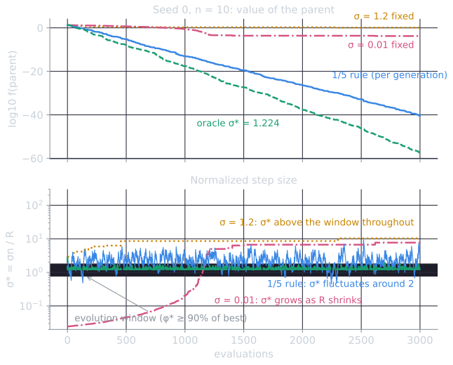
The bottom panel explains the gap between the per-generation rule and the oracle. Over evaluations 300 to 3,000 of this run, the rule's $\sigma^*$ had a median of 2.22, with 90% of values between 1.09 and 4.22. That is about what the success rate predicts. The rule settled at a success rate of 0.161 rather than 0.2, for the reason Auger and Hansen give, and on the asymptotic curve a success probability of 0.161 corresponds to $\sigma^* = 1.98$ and $\varphi^* = 0.168$, 83% of the maximum. The measured rate, 0.161 against the oracle's 0.229 in ten dimensions, is lower again, 70% of the oracle's, since $\sigma^*$ fluctuates widely instead of staying at one value, and the excursions to 3 or 4 make little progress.
Linear convergence
The per-generation rule's median $\log_{10} f$ for $n = 10$ was $-12.8$ after $100n$ evaluations, $-26.7$ after $200n$, and $-40.5$ after $300n$: about 13.9 decimal places of $f$ per $100n$ evaluations, every time. For $n = 30$ the steps were 14.4 and 14.6. This is linear convergence, in the terminology of numerical optimization: the error decreases by a constant factor per iteration, so its logarithm decreases linearly with the number of evaluations. If the normalized rate is $c$, then $\ln R$ falls by $c/n$ per evaluation and $\log_{10} f = 2 \log_{10} R$ falls by $2c / (n \ln 10)$, which is $86.9c$ decimal places per $100n$ evaluations. With $c = 0.161$ that gives 14.0, matching the measured 13.9.
Three things follow. The number of evaluations needed for each additional digit of accuracy is constant. It grows in proportion to $n$, since the rate per evaluation is $c/n$. And no step-size rule can push $c$ above the maximum of $\varphi^*$, about 0.2 for large $n$ and somewhat more in small dimensions.
These are not only simulation results. Jägersküpper analyzed the (1+1)-ES with isotropic mutations on the sphere and on convex quadratic functions and proved linear convergence with overwhelming probability, with a convergence rate of order $1/n$ (Jägersküpper, 2006, and earlier papers, as summarized by Glasmachers, 2020). Akimoto, Auger, and Glasmachers (2018) gave non-asymptotic bounds on the expected time for the (1+1)-ES with the 1/5 success rule to reach a target on the sphere, again with a convergence rate of order $1/n$. Auger and Hansen (2016) developed a general method for proving linear convergence of comparison-based algorithms with step-size adaptation on scaling-invariant functions, with the (1+1)-ES with the generalized 1/5 rule as one of their examples. The underlying reason is invariance. The algorithm uses only comparisons of $f$ values, and on the sphere the problem looks the same at every scale, so if $\sigma$ stays in proportion to $R$, every generation is a scaled copy of the previous one.
The limitation: one step size for all directions
The 1/5 rule adapts a single number. It can make the mutation distribution larger or smaller, but not change its shape. On the ellipsoid
$$f(\mathbf{x}) = \sum_{i=1}^{n} \kappa^{(i-1)/(n-1)} \, x_i^2,$$
whose curvature differs by a factor $\kappa$ between the flattest axis ($i = 1$) and the steepest ($i = n$), the step size that gives a success probability of 1/5 is set by the steep directions, and it is far too small for the flat ones. Same script, $n = 10$, per-generation rule, 30 runs, budget one million evaluations:
| Condition number $\kappa$ | Evaluations to $f \le 10^{-8}$ | Late rate (decades of $f$ per 1,000 evaluations) | Success rate |
|---|---|---|---|
| 1 (sphere) | 664 (630–690) | 13.9 | 0.162 |
| $10^2$ | 4,265 (4,056–4,528) | 1.94 | 0.194 |
| $10^4$ | 225,754 (218,170–234,272) | 0.038 | 0.200 |
| $10^6$ | not reached in $10^6$ | 0.0010 | 0.200 |
The late rate is measured between $f = 10^{-8}$ and $10^{-20}$, or over the second half of the budget for runs that did not get there. Every run still converged linearly, and the success rate stayed at the target. The rule did exactly what it was designed to do, and the convergence rate fell by a factor of about 7 at $\kappa = 10^2$, about 360 at $10^4$, and about 14,000 at $10^6$. With $\kappa = 10^6$ the median $f$ after a million evaluations was $10^{-0.2}$. At the end of those runs the parent was a median of about 800,000 times farther from the optimum along the flattest axis than along the steepest: the search had converged in the steep directions and was crawling along the flat one. At the late rate measured, another eight decades would take on the order of ten million evaluations.
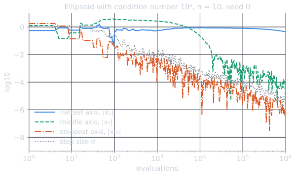
The figure shows the mechanism in one run. A mutation changes $f$ by a gain along the gradient, linear in $\sigma$, minus a cost $\sigma^2 \sum_i \kappa_i z_i^2$, which is quadratic in $\sigma$ and dominated by the steepest directions, the same balance as in the derivation for the sphere. Holding the success rate at 1/5 keeps the two comparable, which pins $\sigma$ near the size of the gradient divided by the largest curvature. At the end of this run $\sigma$ was $1.3 \times 10^{-6}$, while the flattest coordinate, which by then accounted for about two thirds of $f = 0.298$, was still 0.45 from the optimum: steps of that size move it by a few millionths per generation. In this run $|x_{10}|$ fell from $10^{0.24}$ to $10^{-5.9}$ over a million evaluations, $|x_5|$ from $10^{0.10}$ to $10^{-5.7}$, and $|x_1|$ only from $10^{-0.26}$ to $10^{-0.35}$.
Beyer and Schwefel (2002, §4.2) list the rule's other restrictions. It controls a single strategy parameter. It requires that the success probability exceed 1/5 for small enough step sizes; where it does not, $\sigma$ keeps shrinking and the search stagnates prematurely (Schwefel, 1995, pp. 116 f., as cited there). A parent near the tip of a narrow feasible cone is an example of our own: for every $\sigma$, only a small fraction of directions are both feasible and improving. And it is usually used only in the (1+1)-ES, since other strategies have different optimal success probabilities. Glasmachers (2020) characterizes the functions on which the (1+1)-ES with success-based step-size control converges to a critical point, and shows that it can converge prematurely with positive probability on some others.
Where the idea leads
Each limitation has a successor. Strategies with populations adapt the step size through selection itself, by attaching $\sigma$ to each individual and letting it evolve, and can adapt one step size per coordinate, which solves the axis-parallel ellipsoid above; see $(\mu,\lambda)$ selection and self-adaptation. CMA-ES adapts a full covariance matrix, which handles ellipsoids in any orientation, and uses an evolution path rather than a success count to set the overall step size. The success rule itself remains a cheap step-size control for elitist strategies with a single offspring, and Kern et al. (2004) included a (1+1)-ES of this kind in their comparison of continuous evolutionary algorithms. The general evolution strategies topic places these methods side by side.
References
- Akimoto, Y., Auger, A., and Glasmachers, T. (2018). Drift theory in continuous search spaces: Expected hitting time of the (1+1)-ES with 1/5 success rule. In Proceedings of the Genetic and Evolutionary Computation Conference (GECCO '18), 801–808. ACM.
- Auger, A., and Hansen, N. (2016). Linear convergence of comparison-based step-size adaptive randomized search via stability of Markov chains. SIAM Journal on Optimization, 26(3), 1589–1624.
- Beyer, H.-G., and Schwefel, H.-P. (2002). Evolution strategies: A comprehensive introduction. Natural Computing, 1(1), 3–52.
- Eiben, A. E., and Smith, J. E. (2015). Introduction to Evolutionary Computing, 2nd ed. Springer.
- Glasmachers, T. (2020). Global convergence of the (1+1) evolution strategy to a critical point. Evolutionary Computation, 28(1), 27–53.
- Jägersküpper, J. (2006). How the (1+1) ES using isotropic mutations minimizes positive definite quadratic forms. Theoretical Computer Science, 361(1), 38–56.
- Kern, S., Müller, S. D., Hansen, N., Büche, D., Ocenasek, J., and Koumoutsakos, P. (2004). Learning probability distributions in continuous evolutionary algorithms: A comparative review. Natural Computing, 3(1), 77–112.
- Rechenberg, I. (1973). Evolutionsstrategie: Optimierung technischer Systeme nach Prinzipien der biologischen Evolution. Frommann-Holzboog.
- Schumer, M., and Steiglitz, K. (1968). Adaptive step size random search. IEEE Transactions on Automatic Control, 13(3), 270–276.
- Schwefel, H.-P. (1975). Evolutionsstrategie und numerische Optimierung. Doctoral dissertation, Technical University of Berlin.
- Schwefel, H.-P. (1995). Evolution and Optimum Seeking. Wiley.