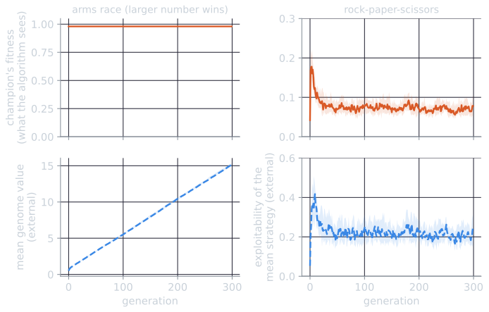
Two runs of a coevolutionary algorithm produce equally uninformative fitness curves. In each, a population of 50 strategies plays a two-player game, every individual plays every other, and the best individual's average score shows no upward trend over the last 200 generations. In the first run the strategies are numbers, and the larger number wins; by the end the population's average value has grown from 0.5 to about 15, and later champions almost always beat earlier ones. In the second run the game is rock-paper-scissors; the population rotates from rock to paper to scissors and back about 17 times, and the final champion is no better than the first. The fitness curve does not tell the runs apart, because in both the opponents improve, or change, as fast as the individual being measured.
This is the problem the name Red Queen has come to stand for in evolutionary computation. Fitness in a competitive coevolutionary algorithm is measured against other evolving individuals, so it is relative, and a constant relative fitness can hide steady progress, endless cycling, or stagnation. This article starts from the biological hypothesis that gave the effect its name, uses the Lotka-Volterra predator-prey equations as an analogy for coupled oscillation, describes the failure modes of coevolutionary algorithms (cycling, disengagement, forgetting and mediocre stable states), and then covers the methods that have been proposed to measure progress when fitness cannot. A small experiment, tools/experiments/evolution/red_queen.py in the site repository, produces every number quoted for the two runs above.
The Red Queen hypothesis in biology
Leigh Van Valen compiled published data on how long fossil taxa had lasted, across groups from foraminifera to mammals, and plotted, for each group, how many taxa survived for a given length of time. On a logarithmic scale the survivorship curves were close to straight lines. A straight line means that the probability that a taxon goes extinct in the next interval does not depend on how long it has already existed: an old genus is as likely to disappear as a young one. Van Valen (1973) stated this as a law of constant extinction, and proposed an explanation for it. The effective environment of any group of organisms deteriorates at a stochastically constant rate, and he attributed the deterioration mainly to other species rather than to the physical environment. Every improvement in a species' predators, prey, competitors or parasites makes its own environment worse, so a species must keep evolving merely to hold its position. Van Valen framed the interactions within an adaptive zone as approximately zero-sum: one species' gain is another's loss. He named the idea after the Red Queen in Lewis Carroll's Through the Looking-Glass (1871), who tells Alice, "Now, here, you see, it takes all the running you can do, to keep in the same place."
Two points matter for what follows. Van Valen's claim was about extinction rates in the fossil record, a law with exceptions, as Solé (2022) notes in a retrospective, and the Red Queen was his explanation for it. And the hypothesis concerns a lineage's chance of persisting, which stays roughly constant while the organisms keep changing; it does not say whether the changes accumulate. An arms race, in which predators and prey both become steadily faster, and a cycle, in which traits come and go, are both consistent with it. That ambiguity is what makes coevolutionary algorithms hard to monitor.
Predator and prey: the Lotka-Volterra analogy
The classic picture of two species pushing each other around is the predator-prey model of Lotka (1925) and Volterra (1926). With $x$ prey and $y$ predators,
$$\frac{dx}{dt} = \alpha x - \beta x y, \qquad \frac{dy}{dt} = \delta x y - \gamma y.$$
The first equation is the prey equation. Without predators the prey grow exponentially at rate $\alpha$; each encounter between a predator and a prey, whose frequency is proportional to $xy$, removes prey at rate $\beta$. The second is the predator equation: predators die at rate $\gamma$ without food and increase at rate $\delta$ per encounter. All four constants are positive.
Setting both derivatives to zero gives an interior equilibrium at $x^* = \gamma/\delta$ and $y^* = \alpha/\beta$. Away from it the populations oscillate. The function
$$V(x, y) = \delta x - \gamma \ln x + \beta y - \alpha \ln y$$
is constant along every solution. Its time derivative is $(\delta - \gamma/x)\,x(\alpha - \beta y) + (\beta - \alpha/y)\,y(\delta x - \gamma) = (\delta x - \gamma)(\alpha - \beta y) - (\alpha - \beta y)(\delta x - \gamma) = 0$. The orbits are therefore closed curves around the equilibrium: each starting point stays on its own cycle forever, which neither spirals into the equilibrium nor out to extinction. The equilibrium is neutrally stable. Linearizing at $(x^*, y^*)$ gives oscillations of angular frequency $\sqrt{\alpha\gamma}$, so small cycles have period $2\pi/\sqrt{\alpha\gamma}$.
The script integrates the equations with the fourth-order Runge-Kutta method (step 0.001, 50 time units) for $\alpha = 1$, $\beta = 0.1$, $\gamma = 1.5$ and $\delta = 0.075$. The equilibrium is $(20, 10)$, and the small-oscillation period is $2\pi/\sqrt{1.5} = 5.130$.
| Start $(x_0, y_0)$ | Prey range | Predator range | Period | Prey peak to predator peak |
|---|---|---|---|---|
| (10, 5) | 7.93 to 40.60 | 3.09 to 23.28 | 5.480 | 0.898 |
| (15, 8) | 14.17 to 27.24 | 6.52 to 14.54 | 5.187 | 1.104 |
| (19, 10) | 19.00 to 21.03 | 9.39 to 10.64 | 5.132 | 1.252 |
| (20, 10) | stays at 20 | stays at 10 | none | none |
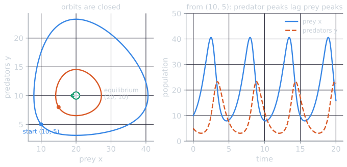
Each orbit keeps the size its starting point gave it, so the amplitude is set by the initial condition and never decays; $V$ drifted by at most $3.4 \times 10^{-14}$ of its value. Large cycles are slower than the linear prediction, and near the equilibrium the period approaches 5.130. Predator peaks follow prey peaks; close to the equilibrium the lag approaches a quarter period ($5.130/4 \approx 1.28$).
The model is an analogy for coevolutionary dynamics, and only an analogy. It describes the numbers of two species, with no heredity, variation or selection on traits; the populations of a coevolutionary algorithm have fixed sizes, and what changes is which strategies they contain. The neutral cycles are also fragile: adding prey self-limitation, for instance, makes the equilibrium attract the orbits. What the analogy does capture is the coupling: each population's growth depends on the other's state, and the delay between them produces oscillation rather than convergence. A precise mathematical relative exists. Hofbauer and Sigmund (1998) show that the replicator equation, the standard model of frequency-dependent selection among $n$ strategies, is equivalent to a Lotka-Volterra system with $n - 1$ species. For rock-paper-scissors the continuous-time replicator equation also has a neutrally stable equilibrium surrounded by closed orbits, while its discrete-time version, which corresponds to fitness-proportional selection in a generational algorithm, spirals away from the equilibrium (Ficici, 2004, §3.5).
Relative fitness hides progress
In an ordinary evolutionary algorithm, fitness is a fixed function of the individual. In a coevolutionary algorithm it is a function of the individual and the opponents or partners it was evaluated with (Eiben and Smith, 2015, ch. 15). Ficici (2004, §3.3) calls the measured quality contextual: in a zero-sum game, a good individual tested against superior opponents looks poor, and a mediocre one tested against poor opponents looks superior. Monitoring the population's mean or best fitness therefore cannot reveal whether behavior is improving. Floreano and Nolfi (1997) describe the same problem from the inside of a predator-prey robotics experiment: progress by one population is achieved at the expense of the other's fitness, and the fitness landscape of each changes continually with its competitor. They call this continual change the Red Queen effect.
Ficici (2004, §3.5) separates the Red Queen from cycling: the need to keep evolving to maintain fitness is present both when strategies cycle and when two populations are in a genuine arms race, and the two situations cannot be told apart by monitoring fitness. The methods described below were developed for this reason.
Pathologies of coevolutionary algorithms
The research literature names a set of recurring failure modes. Ficici (2004, ch. 3) reviews them one by one, and Popovici, Bucci, Wiegand and de Jong (2012) survey them in a broader account of coevolutionary algorithms.
Cycling in intransitive games. A superiority relation is intransitive when A beats B and B beats C, yet C beats A. Rock-paper-scissors is the smallest example. Its only Nash equilibrium is to play each move with probability $1/3$, but a population that drifts toward rock rewards paper, a population of paper rewards scissors, and so on. Selection favors whatever beats the current majority, and the population chases its own tail. Ficici lists reported cycles in cellular-automaton classification, time-series prediction, and pursuit and evasion (Ficici, 2004, §3.5.1).
Disengagement and loss of gradient. Selection needs differences in fitness. If no test can distinguish between the individuals being tested, the search has lost its gradient; when the tests come from a second population, the two populations are said to be disengaged. The typical case is a two-population system in which one side becomes so much stronger that every one of its members beats every member of the other. Then every individual in both populations receives the same score, selection becomes uniform random, and both populations drift. In the "numbers games" of Watson and Pollack (2001), minimal two-population games designed to make these dynamics visible, the drift eventually brings the populations back into contact, but at the cost of losing traits (Ficici, 2004, §3.4.1). Proposed remedies include slowing the stronger population until the weaker catches up and rewarding moderate rather than total success against opponents (Ficici, 2004, §3.4.2).
Forgetting. A trait is forgotten when the population loses it and later would benefit from having it again. Ficici (2004, §3.6) distinguishes three causes. The trait may be selected against, which is the intransitive cycle again. It may be selectively neutral and lost to drift because selection pressure has become too narrow; Watson and Pollack (2001) call this focusing. Or it may be selected for but hard to keep, which points to a missing elitism mechanism.
Mediocre stable states. Pollack and Blair (1998) gave this name to a self-learning system that settles into an equilibrium of its own learning dynamics without becoming good at the task: a student and a teacher that narrow the game to a style both can handle, aim for draws, or collude, for example by throwing alternate games. Their hypothesis was that backgammon resists such states because the dice make every position reachable and keep either player from narrowing the game. A mediocre stable state is the static counterpart of cycling: the fitness record is flat because nothing is changing, not because everything is.
Solution concepts. Ficici's thesis argues that these pathologies are symptoms of a single underlying problem. A solution concept specifies which individuals, or which sets or mixtures of individuals, count as solutions in an interactive domain. Every coevolutionary algorithm implements some solution concept, by design or by accident, and the pathologies appear when the implemented concept differs from the one the experimenter intended (Ficici, 2004). Ficici argues, for example, that the standard replicator dynamics implement no solution concept at all for rock-paper-scissors, since they never converge, and reads cycling as a sign that a solution concept has been implemented improperly (Ficici, 2004, §3.5). The Nash equilibrium and the set of Pareto-nondominated individuals, both discussed below, are two explicit solution concepts that algorithms have been built around.
Experiment: coevolving rock-paper-scissors
The experiment shows cycling and the measurement problem in the simplest setting where they occur. Both games are symmetric and zero-sum, and both use the same algorithm: one population of $N = 50$ individuals, every individual plays every member of the population, its fitness is its mean payoff, parents are chosen by binary tournament, and each child is mutated by adding Gaussian noise with $\sigma = 0.05$. There is no crossover and no elitism. Each game was run for 300 generations with 30 seeds; results are medians with interquartile ranges.
- Rock-paper-scissors. An individual is a mixed strategy $p = (p_R, p_P, p_S)$, a probability for each move. The payoff to $p$ against $q$ is the expected score $p^\top A q$, where $A$ gives 1 for a win, $-1$ for a loss and 0 for a draw. Negative probabilities after mutation are set to zero and the vector is renormalized.
- Arms race. A transitive control, a one-dimensional numbers game: an individual is a real number $x$, and $x$ beats $y$ whenever $x > y$ (payoff 1 for a win, $-1$ for a loss, 0 for a tie).
Since every individual's fitness is its mean payoff against the population, and both games are zero-sum, the population's mean fitness is exactly zero in every generation of both games. The reason takes one line. With payoffs antisymmetric, $u(q, p) = -u(p, q)$, the mean fitness is $\frac{1}{N^2}\sum_i \sum_j u(p_i, p_j)$, and every term $u(p_i, p_j)$ is cancelled by its partner $u(p_j, p_i)$, while the diagonal terms $u(p_i, p_i)$ are zero. Whatever the population does, the average individual breaks even. The best individual's fitness is what an experimenter would plot, and it says almost nothing. In the arms race it is 0.980 in every generation (the champion beats all 49 others and ties itself). In rock-paper-scissors it averages 0.078 [0.071, 0.085] over generations 100 to 199 and 0.073 [0.069, 0.078] over generations 200 to 299.
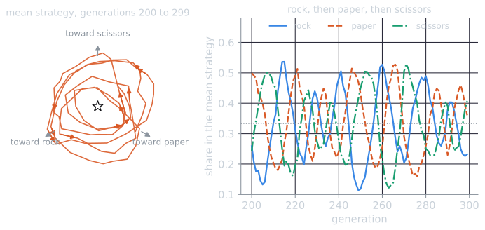
External measures, which the algorithm never sees, tell the two runs apart. In the arms race the mean genome value climbs from 0.503 [0.486, 0.522] to 15.145 [14.965, 15.320]. In rock-paper-scissors the useful external measure is the exploitability of the population's mean strategy $m$: the most that an opponent choosing its best response could win per game against $m$. It is 0 at the Nash equilibrium and 1 for a pure strategy. Over generations 100 to 299 it averages 0.225 [0.214, 0.238], and it does not fall. Instead the mean strategy circles the equilibrium, making 17.2 [16.2, 18.0] full turns in 300 generations, about one turn every 17 generations, always in the direction rock to paper to scissors. In seed 0 the mean strategy is 48% rock at generation 240, 43% paper at 244, 50% scissors at 252, and 53% rock again at 260. Neither the neutral orbits of the continuous replicator equation nor the outward spiral of the discrete one describes this run, which is our own observation: mutation pulls the population toward the centre of the simplex, selection pushes it outward, and the cycle settles at a noisy, roughly constant amplitude.
Experiment: two populations, engaged and disengaged
The one-population arms race shows progress hidden by relative fitness. A two-population version shows it from a different side, and adds the opposite failure. In tools/experiments/evolution/red_queen_extra.py, a minimal two-population numbers game in the spirit of Watson and Pollack (2001), with details of our own, hosts and parasites are real numbers and a host beats a parasite when its number is larger. Each population has 50 members, every host meets every parasite, and each individual's fitness is the fraction of the other population it beats. Each population is then replaced by binary tournament selection and Gaussian mutation with $\sigma = 0.05$, for 300 generations and 30 seeds. Two starts are compared: both populations uniform on $[0, 1)$, and parasites uniform on $[3, 4)$, so that every parasite beats every host from the first generation.
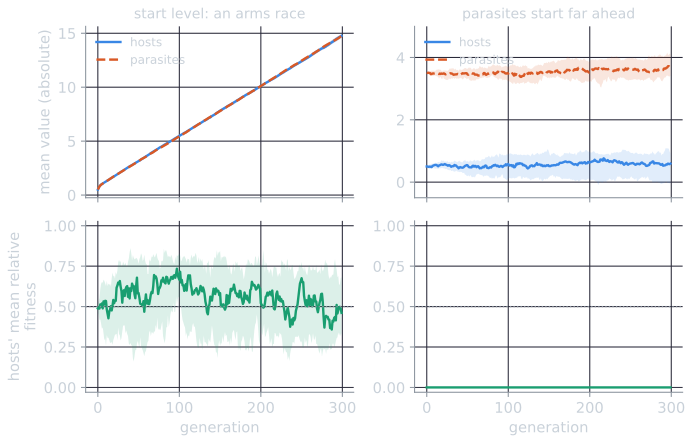
From the level start, the arms race of the one-population game reappears with two populations. The hosts' mean value rises from 0.503 [0.486, 0.522] to 14.758 [14.534, 14.922], the parasites' from 0.510 to 14.739, and the two medians stay within a few hundredths of each other. Meanwhile the hosts' mean relative fitness, averaged over generations 50 to 299, is 0.549 [0.437, 0.629]. Individual runs swing much more than the median suggests. In seed 0 the hosts' mean relative fitness ranges from 0.02 to 1.00 after generation 50, and across runs the longest spell with one side ahead lasts a median of 86.5 generations (54 to 152). Yet the largest gap between the two population means in seed 0 after generation 50 is 0.32, about six times the mutation's standard deviation: a lead that relative fitness reports as total dominance is, in absolute terms, small. Both populations improve by about 0.05 per generation in absolute terms, and their relative fitness says nothing about it. This is the Red Queen in its plainest form.
From the separated start, the populations are disengaged. Every host loses every contest, so every host has fitness 0, every parasite has fitness 1, and binary tournament selection on equal fitness picks parents uniformly at random. Both populations drift. After 300 generations the hosts' mean is 0.594 [−0.022, 0.931] and the parasites' 3.679 [3.418, 4.108], scarcely changed in the median but more spread out, and only 4 of the 30 runs made contact at any point, those four first at a median of generation 259. The parasites have no reason to improve, since nothing tests them, and the hosts have no way to, since every host scores the same. The relative fitness record is perfectly informative about one thing, that the populations have lost contact, and about nothing else.
The demo runs the same game one seed at a time. With equal mutation sizes and no head start it reproduces the arms race; giving the parasites a head start of 3 reproduces disengagement. Making one population's mutations larger than the other's lets that side pull ahead, and with enough difference the populations disengage on their own after starting level. In red_queen_extra.py, with host mutations of $\sigma = 0.02$ and parasite mutations of $\sigma = 0.2$ from a level start, the hosts' mean relative fitness averaged over generations 50 to 299 was 0.004 [0.003, 0.006], the populations were engaged in a median of a third of the generations, and only 3 of 30 runs were engaged at the end. The parasites' mean reached 5.836 against the hosts' 2.821: the faster side ran away and the contest stopped teaching either side anything.
Measuring progress
CIAO plots
Cliff and Miller (1995) proposed testing the best individual of each generation against the best opponents of every earlier generation, which they called current individual vs. ancestral opponents (CIAO). The results form a lower-triangular matrix $C$, with $C[g, h]$ the score of generation $g$'s champion against generation $h$'s, for $h \le g$. If coevolution is making progress, later champions should beat earlier ones, and the matrix should fill with wins below the diagonal. Floreano and Nolfi (1997) applied the method to their predator and prey robots and described their CIAO plots as "Scottish tartan" patterns: periods of relative stasis interrupted by short, radical changes of behavior.
The CIAO matrix for rock-paper-scissors, seed 0, every fourth generation from 240 to 268:
| $g$ \ $h$ | 240 | 244 | 248 | 252 | 256 | 260 | 264 | 268 |
|---|---|---|---|---|---|---|---|---|
| 240 | 0 | |||||||
| 244 | 0.17 | 0 | ||||||
| 248 | 0.00 | 0.09 | 0 | |||||
| 252 | −0.13 | 0.07 | 0.07 | 0 | ||||
| 256 | −0.17 | −0.02 | 0.09 | 0.08 | 0 | |||
| 260 | 0.22 | −0.19 | −0.12 | 0.05 | 0.21 | 0 | ||
| 264 | 0.23 | −0.09 | −0.12 | −0.03 | 0.11 | 0.13 | 0 | |
| 268 | −0.15 | 0.18 | 0.08 | −0.07 | −0.19 | 0.07 | 0.16 | 0 |
Each champion beats the champions of the last few generations and loses to some older ones, and the bands of positive and negative entries run roughly parallel to the diagonal. The champion of generation 260, which plays rock 47% and paper 48% of the time, beats the rock-heavy champion of generation 240 (72% rock) by 0.22 per game, and loses by 0.19 to the champion of generation 244, which plays mostly paper and scissors. In the same run, averaged over generations 100 to 299, the score against the champion $k$ generations back is positive for $k = 1$ to 9 (largest, 0.12, at $k = 4$ and 5), about zero at $k = 10$, negative from $k = 11$ to 20 (lowest, $-0.06$, at $k = 14$ to 16), and within $\pm 0.02$ beyond that. Over the 30 runs, the mean of all entries below the diagonal is 0.003 [0.003, 0.004]: the champions as a whole beat their ancestors no more often than they lose to them. In the arms race every entry below the diagonal in the same window of seed 0 is 1.00, and the mean over all pairs is 0.999 [0.998, 0.999].
Drawn as images, the two matrices look nothing alike, and this is how CIAO plots are meant to be read. Each row is one champion; each cell to the left of the diagonal is its score against an ancestor.
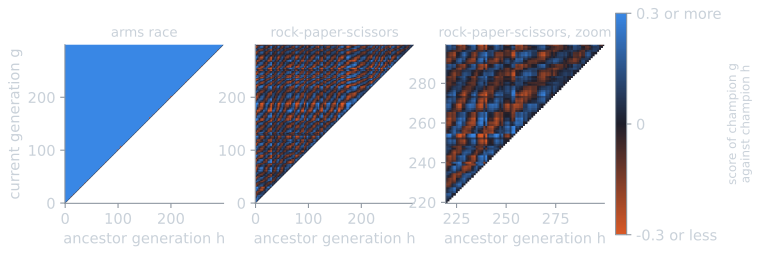
A solid lower triangle is the signature of steady progress; stripes parallel to the diagonal are the signature of a cycle, since they mean that the outcome depends on the lag $g - h$ alone; and a lower triangle that fades from colour near the diagonal to neutral far from it would mean that champions beat their recent ancestors but not their distant ones, which is the pattern forgetting would be expected to leave.
Master tournaments
Floreano and Nolfi (1997) used a master tournament: each generation's best individual is tested against the best competitors of all generations, and its average score is its master fitness. The method answers a practical question that the fitness record cannot, namely which generation produced the best individuals, which in a coevolutionary run need not be the last. In the experiment, the master fitness of the final champion minus that of the first is 1.993 [1.993, 1.993] in the arms race, against a maximum possible difference of 2, and 0.002 [−0.007, 0.019] in rock-paper-scissors, where every champion's master fitness stays within a few hundredths of zero.
The arms-race figure can be worked out by hand. If every champion beats all earlier champions and loses to all later ones, the champion of generation $g$ (counting from 0, with $G = 300$ generations) wins $g$ games, ties itself, and loses $G - 1 - g$. Its master fitness is
$$\frac{g - (G - 1 - g)}{G} = \frac{2g - G + 1}{G},$$
which rises in a straight line from $-299/300 = -0.997$ for the first champion to $+0.997$ for the last. The difference is $598/300 = 1.993$, the value measured. The bound of 2 is out of reach only because each champion ties itself.
A master tournament ranks individuals by how many collected opponents they beat, which hides intransitivity. Stanley and Miikkulainen (2004) point out that if strategy A beats 499 of 500 opponents and B beats 498, the master tournament ranks A above B even if B beats A head-to-head.
Dominance tournaments
Stanley and Miikkulainen (2004) describe a stricter alternative, the dominance tournament, which they used to monitor coevolution of neural-network controllers evolved with NEAT in a robot duel. The first generation's champion is the first dominant strategy. A later generation's champion becomes the next dominant strategy only if it beats every dominant strategy found so far. The resulting sequence contains no cycles by construction, so each new level is strictly better than all earlier levels in head-to-head play, and evaluating a candidate can stop at its first loss, which makes the method cheaper than a master tournament. In their experiments, 13 runs reached between 11 and 19 dominance levels in 500 generations.
In the experiment a champion is counted as beating a dominant strategy when its payoff exceeds 0.01. The arms race produces 270 [267, 271.75] dominant strategies, the last one in generation 299 in every run. Rock-paper-scissors produces 8 [6, 9], the last one at generation 67 [37, 111]: once a few levels exist, any new champion that beats the latest one loses to an earlier one, and the hierarchy stops growing even though the population keeps moving.
The dominance tournament has a known weakness of its own. Ficici (2004, ch. 8) shows, in one of Watson and Pollack's numbers games, that the sequence of dominant strategies converges onto a strategy that is itself dominated by the Nash equilibrium, because the Nash strategy only ties that strategy rather than beating it, and so can never enter the hierarchy. A strict monitoring criterion avoids false progress but can also miss real progress.
Remedies: memory, Pareto coevolution and archives
Memory. Most remedies for forgetting and cycling keep a record of good individuals and use it during evaluation. The hall of fame of Rosin and Belew (1997) keeps the best individual of every generation and tests new individuals against a sample of them, so that a strategy which beats only the current population but loses to old champions is penalized. Ficici (2004, §3.6.2) describes most memory mechanisms in the literature as variants of this best-of-generation scheme, differing in how many past champions they keep and how many they sample, and proposes a Nash memory built around the Nash equilibrium as the solution concept (Ficici, 2004, ch. 8).
Pareto coevolution. Ficici and Pollack (2001) treated the opponents an individual meets as separate objectives, in the sense of multi-objective optimization. Instead of summing an individual's results into a single score, Pareto coevolution compares results opponent by opponent, and keeps the individuals that are Pareto-nondominated: no other individual does at least as well against every opponent and strictly better against one. Intransitivity is then not averaged away; an individual that is the only one to beat some opponent stays nondominated. Ficici and Pollack also rewarded tests for distinctions, for revealing a difference between two learners, which addresses disengagement directly; they applied the method to coevolving cellular-automaton rules and initial conditions for a density classification task (Ficici, 2004, §3.4.2 and ch. 7).
A small outcome matrix of our own shows what the change of view does. Four learners face five tests, and an entry of 1 means the learner passes the test (computed by tools/experiments/evolution/red_queen_extra.py):
| T1 | T2 | T3 | T4 | T5 | Total | Dominated by | |
|---|---|---|---|---|---|---|---|
| L1 | 1 | 1 | 0 | 0 | 1 | 3 | L2 |
| L2 | 1 | 1 | 1 | 0 | 1 | 4 | none |
| L3 | 0 | 0 | 0 | 1 | 1 | 2 | none |
| L4 | 1 | 0 | 1 | 0 | 1 | 3 | L2 |
Summing the rows ranks L2 first and L3 last, and a selection scheme that keeps the top half would discard L3. Compared test by test, L2 passes everything L1 and L4 pass and one more test each, so it dominates both; but nothing dominates L3, which is the only learner to pass T4. Pareto coevolution keeps $\{L2, L3\}$: the best all-round learner and the one with a skill no other learner has. On the test side, T5 is passed by everyone and so distinguishes no pair of learners; T2 and T3 each distinguish 4 of the 6 pairs, and T1 and T4 3 each. A test like T5, however easy to pass, carries no information for selection, which is the same observation Hillis made about random test cases that every network sorted (see competitive coevolution).
Archives with guarantees. De Jong's Incremental Pareto-Coevolution Archive (IPCA) keeps an archive of nondominated learners together with a test archive to which a test is added when it reveals a new distinction between learners. For Pareto coevolution, the archive's quality never decreases, and any detectable improvement can enter it (de Jong, 2004a). The cost is size: since no tests are removed, the test archive grows throughout the run, and de Jong leaves bounding it as an open question. The Layered Pareto-Coevolution Archive (LAPCA) bounds the archive by keeping only a fixed number of Pareto layers of learners (de Jong, 2004b).
Limits
The Red Queen is a useful name for a measurement problem and an imprecise one for anything more. Van Valen's hypothesis concerned extinction rates of real lineages, and the Lotka-Volterra equations concern population sizes; neither says anything specific about strategies in a coevolutionary algorithm. The precise statements are game-theoretic: relative fitness cannot by itself show progress, intransitive games produce cycles under selection, and whether a run is improving depends on the solution concept that defines improvement. The monitoring methods trade cost against reliability: CIAO and master tournaments need a number of games quadratic in the number of generations, and master fitness averages over cycles, while dominance tournaments are cheaper and cycle-free but can stall on a dominated strategy. The experiment here is deliberately small, with three pure strategies and exact expected payoffs; real applications sample opponents and evaluate noisily, and must also decide how much of the evaluation budget to spend measuring the present population rather than searching for a better one.
References
- Carroll, L. (1871). Through the Looking-Glass, and What Alice Found There. Macmillan.
- Cliff, D., and Miller, G. F. (1995). Tracking the red queen: Measurements of adaptive progress in co-evolutionary simulations. In Advances in Artificial Life: Third European Conference on Artificial Life (ECAL 1995), Lecture Notes in Computer Science 929, 200–218. Springer.
- de Jong, E. D. (2004a). The incremental Pareto-coevolution archive. In Genetic and Evolutionary Computation, GECCO 2004, Lecture Notes in Computer Science 3102, 525–536. Springer.
- de Jong, E. D. (2004b). Towards a bounded Pareto-coevolution archive. In Proceedings of the 2004 Congress on Evolutionary Computation, 2341–2348. IEEE.
- Eiben, A. E., and Smith, J. E. (2015). Introduction to Evolutionary Computing, 2nd ed., chapter 15. Springer.
- Ficici, S. G. (2004). Solution Concepts in Coevolutionary Algorithms. Doctoral dissertation, Brandeis University.
- Ficici, S. G., and Pollack, J. B. (2001). Pareto optimality in coevolutionary learning. In Advances in Artificial Life: Sixth European Conference on Artificial Life (ECAL 2001), Lecture Notes in Computer Science 2159, 316–325. Springer.
- Floreano, D., and Nolfi, S. (1997). God save the red queen! Competition in co-evolutionary robotics. In J. R. Koza et al. (eds.), Genetic Programming 1997: Proceedings of the Second Annual Conference, 398–406. Morgan Kaufmann.
- Hofbauer, J., and Sigmund, K. (1998). Evolutionary Games and Population Dynamics. Cambridge University Press.
- Lotka, A. J. (1925). Elements of Physical Biology. Williams and Wilkins.
- Pollack, J. B., and Blair, A. D. (1998). Co-evolution in the successful learning of backgammon strategy. Machine Learning, 32(3), 225–240.
- Popovici, E., Bucci, A., Wiegand, R. P., and de Jong, E. D. (2012). Coevolutionary principles. In G. Rozenberg, T. Bäck, and J. N. Kok (eds.), Handbook of Natural Computing, 987–1033. Springer.
- Rosin, C. D., and Belew, R. K. (1997). New methods for competitive coevolution. Evolutionary Computation, 5(1), 1–29.
- Solé, R. (2022). Revisiting Leigh Van Valen's "A New Evolutionary Law" (1973). Biological Theory, 17, 120–125.
- Stanley, K. O., and Miikkulainen, R. (2004). Competitive coevolution through evolutionary complexification. Journal of Artificial Intelligence Research, 21, 63–100.
- Van Valen, L. (1973). A new evolutionary law. Evolutionary Theory, 1, 1–30.
- Volterra, V. (1926). Fluctuations in the abundance of a species considered mathematically. Nature, 118, 558–560.
- Watson, R. A., and Pollack, J. B. (2001). Coevolutionary dynamics in a minimal substrate. In L. Spector et al. (eds.), Proceedings of the Genetic and Evolutionary Computation Conference (GECCO 2001), 702–709. Morgan Kaufmann.