Suppose we want a convolutional network for CIFAR-10, and we have decided its outer skeleton: a stem, three stacks of repeated cells, downsampling between stacks, a classifier at the end. What remains is the cell. It is a small directed graph whose vertices apply operations such as a 3×3 convolution or a max pool, and the number of ways to wire one is in the hundreds of thousands even when it has only seven vertices. Each candidate costs a full training run to judge, and two training runs of the same candidate give different accuracies. Choosing the cell by search instead of by hand is neural architecture search (NAS).
The early neuroevolution methods covered in this topic, from weight evolution to NEAT, evolve the network itself, weights included, and score it on a task. Architecture search for deep learning splits the work differently. Evolution, or another search method, proposes only the architecture; gradient descent trains its weights; the trained network's validation accuracy is the fitness. The search makes a few thousand proposals at most, and nearly all the computation goes into training them. This article covers the evolutionary methods that made the approach competitive, the reinforcement-learning and weight-sharing methods they were compared with, the evidence that random search is a hard baseline to beat, and the use of evolution for training hyperparameters.
The search problem
Elsken, Metzen and Hutter (2019) describe a NAS method by three choices: the search space of architectures it can express, the search strategy that proposes candidates, and the performance estimation strategy that scores them. Written out, with $f(A, H)$ the validation accuracy of architecture $A$ trained with hyperparameters $H$, the ideal is
$$A^* = \arg\max_{A} f(A, H^*(A)), \qquad H^*(A) = \arg\max_{H} f(A, H),$$
the best architecture when each is trained as well as it can be. Nobody can afford an inner hyperparameter search for every candidate, so in practice one set of training hyperparameters $H$ is fixed for all of them and the search maximizes $f(A, H)$ alone (Ying et al., 2019, §5.1). Three properties of $f$ shape everything that follows. It is expensive: one evaluation is a training run. It is noisy: the same $A$ scores differently on different runs. And it is only a proxy: the accuracy that matters is on held-out test data, which must never guide the search.
The search space matters as much as the search. Most work after 2017 searched over cells that are stacked into a fixed skeleton, rather than over whole networks, which shrinks the space and lets a cell found on a small dataset be reused on a larger one (Zoph et al., 2018).
Reinforcement learning and its cost
The method that made NAS prominent was not evolutionary. Zoph and Le (2017) trained a recurrent network, the controller, to emit architecture descriptions token by token, and updated it with the REINFORCE policy gradient, using each sampled network's validation accuracy as the reward. Their controller trained 12,800 architectures for CIFAR-10, with 800 networks training at once on 800 GPUs, and the best architecture, widened by 40 filters per layer, reached a test error of 3.65%. The follow-up that introduced the cell-based NASNet search space ran on 500 GPUs for four days (Zoph et al., 2018). Those budgets are the backdrop for everything below: they put NAS out of reach of most laboratories, and they made the efficiency of the search strategy a first-order question.
Large-scale evolution
Real et al. (2017) asked whether a simple evolutionary algorithm, given enough hardware, could produce competitive image classifiers with no human input after the start. Each individual was a trained network. A worker repeatedly chose two individuals at random, removed the worse one from the population, and copied and mutated the better one; the child was trained, evaluated on validation data and returned to the population. This is tournament selection with tournaments of two, run asynchronously by many workers sharing a file system, so no worker waits for a generation to finish. Mutations made one change at a time: insert or remove a convolution, change a stride, a filter count or the learning rate, add or remove a skip connection, reset the weights. Children inherited their parent's trained weights wherever the architecture allowed, so later individuals did not start training from scratch.
Populations of 1,000 began from trivial networks with no convolutions at all. Across five runs, each spread over 250 workers, the best model by validation accuracy reached 94.6% test accuracy on CIFAR-10 (95.6% for an ensemble of the top two models from each population), and the runs ended at a mean of 94.1% with standard deviation 0.4%. A single CIFAR-100 run reached 77.0%. The cost was large: about $9 \times 10^{19}$ floating-point operations per CIFAR-10 run, $4 \times 10^{20}$ for all five. Two control experiments isolate the ingredients. With selection disabled, so that individuals were killed and reproduced at random, the best accuracy reached in the same time on the same hardware was 87.3%; with weight inheritance disabled it was 92.2%.
Regularized (aging) evolution
A year later Real, Aggarwal, Huang and Le (2019) searched the same NASNet cell space that the reinforcement-learning work had used, which made the first controlled comparison between the two kinds of search possible. Their algorithm changes one detail of tournament selection, and the change is the whole method.
- Initialize. Train $P$ random architectures and put them in a queue, oldest first.
- Select. Draw $S$ members uniformly at random, with replacement. The one with the highest validation accuracy is the parent.
- Vary. Copy the parent's architecture and apply one random mutation: rewire one input of an operation, replace one operation, or, with a small probability, leave it unchanged.
- Replace. Train the child, append it to the queue, and remove the oldest member, whatever its accuracy.
- Repeat steps 2 to 4 until the budget of trained models is spent, and return the most accurate model seen.
The usual way to keep the population at size $P$ is to remove the worst member of the sample; the paper calls that non-aging evolution. Under aging, every model dies after $P$ further cycles, so a lineage persists only if its architecture keeps producing accurate children.
The difference in lifetimes is easy to work out. Under aging the population is a queue: a model enters at the back, moves forward one place per cycle, and leaves at the front after exactly $P$ cycles, whatever its accuracy. Under non-aging evolution a model leaves only when it is drawn into a cycle's sample and is the worst of that sample. With the settings of the experiment below, a sample of $S = 10$ drawn with replacement from $P = 100$, a given member is drawn in a cycle with probability $1 - (1 - 1/P)^S = 1 - 0.99^{10} = 0.0956$, and even then it leaves only if every other member drawn scored higher. The member with the highest observed accuracy is never the worst of a sample that contains any other member, so, short of a sample made of ten copies of it, it never leaves at all, and members near the top leave very rarely. Non-aging evolution keeps its best-scoring models indefinitely; aging gives every model the same fixed lifetime. The authors' explanation is a conjecture, labeled as such. Training is noisy, so some models score well by luck. Under non-aging evolution a lucky model can stay in the population indefinitely and keep winning tournaments. Under aging it must be retrained in the form of its descendants, and an architecture that only got lucky once disappears. The name regularized refers to this resistance to fitting the noise. Their evidence for it is indirect: small-scale experiments on grayscale CIFAR-10 and other datasets in which aging tended to do better than non-aging, and a toy problem (bit strings with Gaussian noise added to the score) in which aging was never worse and pulled ahead as the dimension grew.
The paper's headline results: AmoebaNet-A, the evolved cell scaled up, reached 83.9% top-1 and 96.6% top-5 accuracy on ImageNet. Each search experiment trained 20,000 models on 450 K40 GPUs over about seven days, with $P = 100$ and $S = 25$. In five repeats of each method on CIFAR-10, evolution found more accurate models than reinforcement learning in the early part of the search; when both ran to 20,000 models they ended with similar accuracy; and both beat random search. The claim is therefore narrower than "evolution beats reinforcement learning": in that search space and at that scale, evolution got there sooner and was simpler to implement.
Weight sharing and one-shot search
Both families above train every candidate separately, which is why their budgets are measured in thousands of GPU-days. Weight sharing removes most of that cost. All candidate architectures are treated as subgraphs of one large network whose weights are trained once and reused, so a candidate is scored by evaluating it with inherited weights instead of training it. ENAS kept a reinforcement-learning controller but sampled subgraphs of one shared model; the authors report finding a recurrent cell in about 10 hours on one GPU and describe the method as more than 1,000 times cheaper than the original NAS (Pham et al., 2018). DARTS made the choice between operations continuous, a softmax-weighted mixture on every edge, so that the architecture weights could be optimized by gradient descent alongside the network weights. Its CIFAR-10 searches cost 1.5 to 4 GPU-days (Liu, Simonyan and Yang, 2019).
The price is that a candidate's score with shared weights is not the accuracy it would reach if trained alone, and how well the two agree became one of the field's central questions. Weight sharing also changes what the search strategy contributes, which is where the random-search baselines come in.
Random search as a baseline
Random search is the standard reference point in hyperparameter optimization. With a fixed budget it often matches or beats grid search, because when only a few hyperparameters matter, random points cover each of them more finely than a grid does (Bergstra and Bengio, 2012). Two studies applied the same scrutiny to NAS, and their findings are often summarized more broadly than they were stated.
Li and Talwalkar (2020) treated NAS as a specialized hyperparameter problem and evaluated two random-search baselines on the Penn Treebank and CIFAR-10 benchmarks. Random search with early stopping performed at least as well as ENAS on both. Random search with weight sharing did better still, reaching a state-of-the-art result on Penn Treebank and a competitive one on CIFAR-10. They also documented how hard published NAS results were to reproduce, because code, seeds and evaluation details were often missing.
Yang, Esperança and Carlucci (2020) benchmarked eight NAS methods on five image datasets, measuring each by its improvement over the average randomly sampled architecture from its own search space. Many methods struggled to beat that average significantly. In the widely used DARTS space they found that training tricks in the evaluation protocol had more effect on reported accuracy than the architecture, that the accuracy range of the space was narrow enough for the random seed to reorder rankings, and that the hand-designed macro-structure, the overall wiring of the network, mattered more than the operations the search chose.
Neither paper shows that search is useless. They show that in the engineered, cell-based spaces common at the time, a well-designed space and training recipe produce good networks almost regardless of the search, so a method's reported accuracy says little about its search strategy unless it is compared with random search under the same protocol. Where every candidate is trained separately, the picture is different. On the NAS-Bench-101 table described below, regularized evolution, together with two Bayesian optimization methods (SMAC and BOHB), began to outperform random search after about 25 architectures and reached random search's final quality about five times faster (Ying et al., 2019). The two kinds of result are consistent: random search is strong when the space is easy, and is a baseline that every claim of search efficiency has to clear.
An experiment on NAS-Bench-101
NAS-Bench-101 makes these comparisons cheap. Ying et al. (2019) trained every cell in a compact space three times on CIFAR-10 and published the results. A cell has at most 7 vertices, with input and output fixed and the 5 interior vertices each a 3×3 convolution, a 1×1 convolution or a 3×3 max pool, and at most 9 edges. Up to isomorphism there are 423,624 distinct cells.
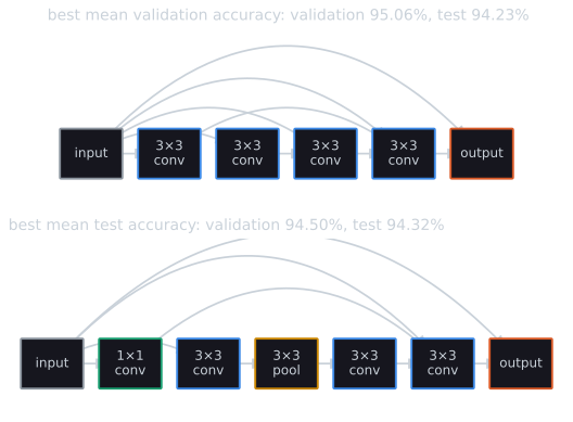
The upper cell shows how the encoding works. The cell is a directed acyclic graph on numbered vertices, written as an upper-triangular adjacency matrix: an entry in row $i$ and column $j$ means the output of vertex $i$ feeds vertex $j$, and only $i < j$ is allowed, which rules out cycles. In the upper cell, edges from the input skip ahead to every interior vertex and to the output, and the last 3×3 convolution also feeds the output. In the benchmark's construction an interior vertex with several inputs sums them, the output vertex concatenates its inputs, and tensors leaving the input vertex are projected to the channel count the next operation expects (Ying et al., 2019, §2.3). The lower cell is the one the paper draws as attaining the lowest mean test error (Ying et al., 2019, Fig. 1), there without its projection layers. The table needs only this matrix and the list of operations to look a cell up, and two matrices that describe the same graph with the vertices numbered differently are the same cell, which is why the count is taken up to isomorphism. A search algorithm that queries the table instead of training gets each answer in microseconds, and the training noise is preserved because each query can return one of the three runs.
The script tools/experiments/evolution/aging_evolution.py in the site repository reads the published 108-epoch table directly (no TensorFlow), checks the benchmark's graph hash for all 423,624 cells, and compares three search strategies over 30 seeded runs each, with a budget of 1,500 queries:
- RS: random cells until the budget is spent.
- RE: aging evolution as above, with $P = 100$ and $S = 10$, the settings Ying et al. used.
- NRE: the same, except that each cycle removes the worst member of the $S$-sample instead of the oldest member of the population.
A random cell has each of the 21 possible edges present with probability 1/2 and each operation uniform, redrawn until valid. A mutation flips each edge with probability 1/7 and changes each operation with probability 1/5. On average that is $21/7 = 3$ edge flips and $5/5 = 1$ operation change per mutation, so a child usually differs from its parent in several places.
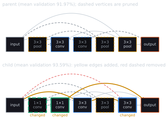
Two features of the encoding show in the figure. Many of the 21 bits can change without changing the computed cell, since edges into or out of pruned vertices do nothing; and a single flip that connects a pruned vertex can change a lot, since it brings that vertex's operation and all its edges into play. Neighbouring encodings therefore sometimes have identical fitness and sometimes very different fitness: the fitness landscape over the 21 bits and 5 operations has both neutral plateaus and abrupt steps. A run's result is the cell with the highest validation accuracy it observed, scored by its test regret: how many percentage points its mean test accuracy falls below that of the best cell in the table, 94.32%. Two evaluation conditions are compared. In the noisy one, each query returns the validation accuracy of one of the three training runs at random, as a real search would see. In the other, each query returns the mean of the three.
Two facts about the table bound what any search can achieve. The cell with the best mean validation accuracy is not the cell with the best mean test accuracy; it scores 94.23% on test, so even a search that finds it has a regret of 0.083 points. And the three training runs of a cell differ in validation accuracy by a median of 0.62 points (interquartile range 0.38 to 0.98), which is wider than most of the differences the search is trying to resolve.
Median test regret in percentage points, with interquartile ranges, over 30 runs:
| Evaluation | Method | 300 queries | 1,500 queries | Found best-validation cell |
|---|---|---|---|---|
| Noisy | RS | 0.738 [0.738, 1.042] | 0.906 [0.619, 1.042] | 0 of 30 |
| RE (aging) | 1.042 [0.738, 1.042] | 0.512 [0.174, 0.576] | 4 of 30 | |
| NRE (non-aging) | 0.738 [0.548, 1.042] | 0.528 [0.238, 0.590] | 2 of 30 | |
| Mean of 3 runs | RS | 0.738 [0.724, 0.738] | 0.461 [0.260, 0.593] | 0 of 30 |
| RE (aging) | 0.324 [0.174, 0.578] | 0.097 [0.097, 0.227] | 7 of 30 | |
| NRE (non-aging) | 0.391 [0.174, 0.734] | 0.097 [0.097, 0.206] | 7 of 30 |
The repeated values in the table (0.738, 1.042, 0.097) are individual cells that many runs end on; the regrets come in steps because the good cells are few. With the Vargha and Delaney (2000) $A$ statistic, the probability that a random run of one method ends with lower regret than a random run of another (0.5 means no difference), the results at 1,500 queries are:
- Evolution beats random search in both conditions: $A = 0.82$ (RE) and $0.75$ (NRE) against RS with noisy evaluations, $0.86$ and $0.87$ with averaged ones.
- Aging and non-aging evolution are indistinguishable here: $A = 0.56$ for RE against NRE with noisy evaluations and $0.47$ with averaged ones. Ying et al. (2019, §4.2) report the ranking RS < NRE < RE over 100 runs with a time budget and a non-aging rule described only as removing the lowest-fitness individual, so this experiment neither confirms nor contradicts them; at this budget, with this mutation and with sample-worst removal, the effect of aging is too small to see in 30 runs.
- Noise makes the final choice unreliable. With noisy evaluations, random search ends worse at 1,500 queries (median 0.906) than at 300 (0.738), and aging evolution's median at 300 queries is worse than at 100 (0.861, printed by the script). The search keeps the single highest observation, and the more cells it scores, the more likely that observation belongs to a cell whose one training run was lucky. Real et al. (2019) argued that aging protects the population from lucky models; nothing in either algorithm, as specified here, protects the final pick. Re-evaluating the top few candidates before choosing would reduce that risk.
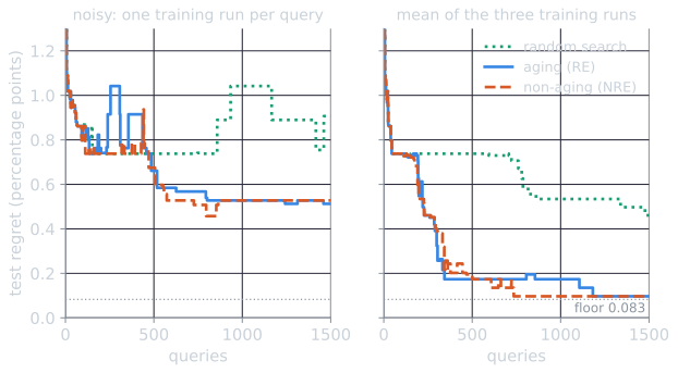
The curves in the figure come from tools/experiments/evolution/aging_evolution_traces.py, which repeats the searches draw for draw and records the pick after every query; its medians at 100, 300 and 1,500 queries are those of the table.
What aging does to lucky models
Real et al.'s (2019) argument for aging is about the population: under non-aging evolution a model that scored well by luck stays and keeps winning tournaments. The traces script measures this directly in the noisy condition. Call a member's luck its observed validation accuracy minus the mean of its cell's three training runs: the part of its score that retraining would not reproduce. A random query has a luck of zero on average.
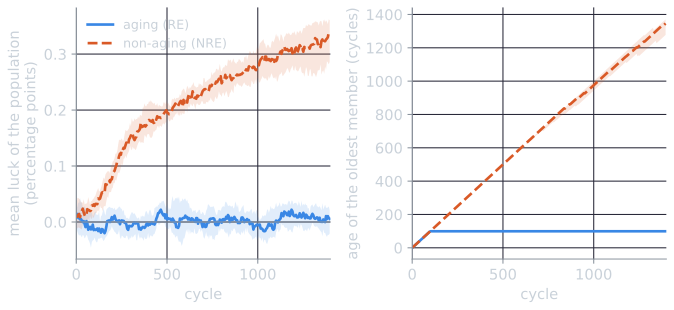
Under aging the population's mean luck stayed at zero throughout: the median over runs was $-0.010$ points after 100 cycles and $0.006$ after 1,400. Under non-aging it grew from 0.029 after 100 cycles to 0.177 after 400 and 0.332 after 1,400 (interquartile range 0.279 to 0.362), about half the median spread of 0.62 points between a cell's three training runs. At cycle 1,400 the oldest member under non-aging evolution had been in the population for a median of 1,341.5 cycles: a model that entered in roughly the first 60 cycles was still there near the end of the run. The selection rule did what the paragraph on lifetimes predicts. Removing the worst of each sample removes the unlucky first, so the survivors become more lucky over time, and their accuracies overstate their cells' quality by more and more.
The luck of the single best-scoring member was about the same under both rules, a median of 0.332 points under aging and 0.497 under non-aging at cycle 1,400, with overlapping interquartile ranges. That is the distinction drawn above. Aging keeps the population honest, so that tournaments compare cells and not luck, but the best observation of a run is a maximum over many noisy draws under either rule. In this experiment, the population-level effect did not translate into a measurably better final pick at 1,500 queries.
The experiment is small by the standards of the papers it follows, and its conclusions are limited to this table. The space is tiny, every cell is trained with one fixed recipe, and a budget of 1,500 queries can reach at most about 0.35% of the space.
Evolving hyperparameters
Architecture is not the only thing evolution can tune during training. Population-based training (PBT; Jaderberg et al., 2017) trains a population of models in parallel, each with its own hyperparameters such as learning rate or entropy cost. Periodically each member is checked. In the variant using truncation selection, a model in the bottom 20% of the population copies the weights and hyperparameters of a model sampled from the top 20% (exploit), then perturbs each hyperparameter by a factor of 0.8 or 1.2, or resamples it from its prior (explore). Because weights are inherited, no training is wasted on restarting, and because hyperparameters change during training, PBT produces a schedule rather than a single setting. Jaderberg et al. reported faster convergence and better final performance on deep reinforcement learning, machine translation and generative adversarial networks.
In the vocabulary of Eiben and Smith (2015, §8.3), PBT is a form of parameter control rather than parameter tuning (ch. 7): it changes hyperparameters while the run proceeds, based on feedback from the population, instead of fixing them in advance. It shares that idea with self-adaptation in evolution strategies and with the dynamic scheduler in the soft-robot project in this topic.
The main alternative for hyperparameters is Bayesian optimization, which fits a probabilistic surrogate model of $f$ to the evaluations so far, usually a Gaussian process, and chooses the next point by maximizing an acquisition function that trades predicted value against uncertainty (Snoek, Larochelle and Adams, 2012). With a few continuous hyperparameters and evaluations too expensive to waste, a surrogate model usually spends the budget better than a population does. Evolution is easier to run in parallel, needs no model of the objective, and handles discrete, conditional and graph-structured spaces naturally, which is why it took hold in architecture search. The distinction is less sharp in practice than in principle. On NAS-Bench-101, SMAC, a Bayesian optimizer with a random-forest surrogate, matched regularized evolution, while TPE, another model-based method, did no better than random search (Ying et al., 2019).
Assessment
Evolution earned its place in architecture search with a modest set of claims. A plain tournament algorithm, scaled up, produced competitive image classifiers from trivial starting points. Aging, a one-line change, gave a method that matched reinforcement-learning search in final quality and reached it sooner in one controlled comparison. And on a tabular benchmark it is among the strongest simple methods. Its costs are those of any search that trains each candidate, and the field's move to weight sharing was driven by cost more than by quality. The random-search studies are a reminder that applies to all of it: the search space and the training recipe determine much of the result, and a search strategy has to be judged against random search under the same protocol, over repeated runs, as the no free lunch results and ordinary significance testing would both suggest.
References
- Bergstra, J., and Bengio, Y. (2012). Random search for hyper-parameter optimization. Journal of Machine Learning Research, 13(10), 281–305.
- Eiben, A. E., and Smith, J. E. (2015). Introduction to Evolutionary Computing, 2nd ed., chapters 7–8. Springer.
- Elsken, T., Metzen, J. H., and Hutter, F. (2019). Neural architecture search: A survey. Journal of Machine Learning Research, 20(55), 1–21.
- Jaderberg, M., Dalibard, V., Osindero, S., Czarnecki, W. M., Donahue, J., Razavi, A., Vinyals, O., Green, T., Dunning, I., Simonyan, K., Fernando, C., and Kavukcuoglu, K. (2017). Population based training of neural networks. arXiv:1711.09846.
- Li, L., and Talwalkar, A. (2020). Random search and reproducibility for neural architecture search. In Proceedings of the 35th Conference on Uncertainty in Artificial Intelligence (UAI 2019), PMLR 115, 367–377.
- Liu, H., Simonyan, K., and Yang, Y. (2019). DARTS: Differentiable architecture search. In International Conference on Learning Representations (ICLR).
- Pham, H., Guan, M., Zoph, B., Le, Q., and Dean, J. (2018). Efficient neural architecture search via parameters sharing. In Proceedings of the 35th International Conference on Machine Learning, PMLR 80, 4095–4104.
- Real, E., Aggarwal, A., Huang, Y., and Le, Q. V. (2019). Regularized evolution for image classifier architecture search. In Proceedings of the AAAI Conference on Artificial Intelligence, 33(01), 4780–4789.
- Real, E., Moore, S., Selle, A., Saxena, S., Suematsu, Y. L., Tan, J., Le, Q. V., and Kurakin, A. (2017). Large-scale evolution of image classifiers. In Proceedings of the 34th International Conference on Machine Learning, PMLR 70, 2902–2911.
- Snoek, J., Larochelle, H., and Adams, R. P. (2012). Practical Bayesian optimization of machine learning algorithms. In Advances in Neural Information Processing Systems 25, 2951–2959.
- Vargha, A., and Delaney, H. D. (2000). A critique and improvement of the CL common language effect size statistics of McGraw and Wong. Journal of Educational and Behavioral Statistics, 25(2), 101–132.
- Yang, A., Esperança, P. M., and Carlucci, F. M. (2020). NAS evaluation is frustratingly hard. In International Conference on Learning Representations (ICLR).
- Ying, C., Klein, A., Christiansen, E., Real, E., Murphy, K., and Hutter, F. (2019). NAS-Bench-101: Towards reproducible neural architecture search. In Proceedings of the 36th International Conference on Machine Learning, PMLR 97, 7105–7114.
- Zoph, B., and Le, Q. V. (2017). Neural architecture search with reinforcement learning. In International Conference on Learning Representations (ICLR).
- Zoph, B., Vasudevan, V., Shlens, J., and Le, Q. V. (2018). Learning transferable architectures for scalable image recognition. In Proceedings of the 2018 IEEE/CVF Conference on Computer Vision and Pattern Recognition, 8697–8710.