Consider two functions on bitstrings of length 20. The first, OneMax, counts the ones. The second, which Droste, Jansen, and Wegener (2002) call Trap, also counts the ones, except that the all-zeros string scores $n + 1 = 21$, more than any other string. Both have a single best point, and they agree everywhere else. Yet a simple evolutionary algorithm that flips random bits and keeps any child at least as good as its parent finds the optimum of OneMax after about 130 evaluations on average, and in 30 runs of 100,000 evaluations each it never finds the optimum of Trap. Every run ends at the all-ones string, the point farthest from the answer.
Nothing about the algorithm changed between the two runs, and the search space is the same. What differs is how fitness is arranged over that space relative to the moves the algorithm can make. The fitness landscape is the standard way to describe that arrangement. This article covers where the idea came from, how it is defined precisely, the features that make a fitness landscape easy or hard to search, and one attempt to summarize hardness in a single number. The experiments are run with the same small algorithm throughout, so the differences come from the problems.
Wright's adaptive landscape
The picture comes from population genetics. Sewall Wright (1932), explaining his theory of evolution to a general audience of geneticists, asked the reader to imagine the field of all possible gene combinations, graded by adaptive value, and drawn as a contour map. High-fitness combinations form peaks, and poor ones form valleys between them. A population occupies a small region of this map, and selection moves it uphill. Wright's question was how a population on a minor peak could ever reach a higher one, since crossing a valley means passing through less fit combinations that selection removes. His answer, the shifting balance theory, relied on small, partly isolated subpopulations in which random drift could carry a population down and across a valley.
Wright was explicit that the two-dimensional diagram is a drastic simplification. The real field of gene combinations has an enormous number of dimensions, one for each locus. The diagram has also been read in two different ways, as a surface over the genotypes of individuals or as mean fitness over the gene frequencies of a population, and its value as a heuristic has been disputed by historians and philosophers of biology (Skipper, 2004).
Evolutionary computation takes the first reading. Each candidate solution is a point, its fitness is the height, and a population is a cloud of points that moves over the surface as it evolves (Eiben and Smith, 2015, ch. 2). Wright's valley-crossing question becomes the central question of search: how an algorithm that mostly accepts improvements escapes a point that is better than everything near it.
A precise definition
The contour map suggests that the search space has a geometry of its own. It does not. A set of bitstrings, permutations, or programs has no built-in notion of which points are close. Closeness comes from the algorithm: two points are neighbors if one variation step can turn one into the other. A fitness landscape is therefore a triple
$$(X, N, f),$$
where $X$ is the set of candidate solutions, $N(x) \subseteq X$ is the set of neighbors of $x$, and $f : X \to \mathbb{R}$ is the fitness function. For bitstrings of length $n$ under single-bit-flip mutation, $N(x)$ is the $n$ strings at Hamming distance 1, and the space has the shape of an $n$-dimensional hypercube.
Jones (1995) made the dependence on the algorithm the center of his account, summarized as "one operator, one landscape": each variation operator induces its own neighborhood structure, and therefore its own fitness landscape, on the same fitness function. The Trap function shows how much this matters. Under single-bit flips, Trap has two local optima, the all-zeros string (the global optimum) and the all-ones string, since every other string can gain fitness by gaining a one. Add a second operator that complements every bit, and the all-ones string becomes a neighbor of the all-zeros string. It is then no longer a local optimum, and the problem is easy. The fitness function did not change, only the moves. The same reasoning explains why the choice between standard binary and Gray coding changes the difficulty of a numeric problem (see binary encoding and Gray codes), and why crossover, which combines two parents, does not fit a simple neighbor graph at all.
Features that make search hard
Local optima and basins
A point $x$ is a local optimum if no neighbor is better: $f(x) \ge f(y)$ for all $y \in N(x)$. Its basin of attraction is the set of starting points from which a strictly improving walk, such as a hill climber, ends at $x$. The number of local optima and the sizes of their basins describe how often a greedy search will stop short. The same structure appears outside evolutionary computation: K-means is a hill climber on the residual sum of squares, and its local minima are why it is restarted from several initial centroids. Mutation in an evolutionary algorithm usually can make larger jumps than a single neighbor step, with small probability, which is one way it escapes (escaping local optima covers the others).
A two-dimensional example makes basins visible, with the caution of Wright's own diagram that two dimensions are not many. Take the square $[0, 1]^2$, divided into a grid of $201 \times 201$ points, each a neighbor of the eight around it, and a fitness made of three smooth hills: a broad one of height 1.00 centered at $(0.25, 0.70)$, a narrower one of height 0.80 at $(0.72, 0.30)$, and a small one of height 0.56 at $(0.75, 0.80)$. A steepest-ascent hill climber moves to the best neighbor until no neighbor is better. Running it from every grid point (the figure script tools/figures/fitness-landscapes.py does this) labels each point with the peak it ends on.
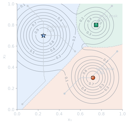
The basin shares turn into a cost. A climber started at a uniformly random point finds the global peak with probability 0.442. Independent restarts fail together with probability $0.558^r$, so the chance of at least one success is 0.688 with two restarts, 0.826 with three and 0.946 with five (rounded to three decimals). Restarting is the simplest cure for local optima, and its cost is set by the size of the best basin, which nobody knows in advance on a real problem. Where basins are many and small, as in the rugged NK fitness landscapes below, restarts become hopeless.
Plateaus and neutrality
A plateau is a connected set of neighboring points with equal fitness. On a plateau, selection provides no direction, and the search drifts at random until it stumbles on an edge. The extreme case is a "needle in a haystack" function, equal everywhere except at one point, where no algorithm can do better than guess. Neutrality is not always harmful. In biology, and in some genetic programming and grammatical encodings, networks of equal-fitness points let a population move a long way without losing fitness, and reach regions from which improvements are possible. Genetic drift, the random change that dominates when selection provides no direction, is treated in natural selection for computer scientists.
A block function shows neutrality at work. Split a string of 32 bits into eight blocks of four, and let fitness be the number of blocks that are all ones. A block with three ones scores the same as a block with none, so almost every point lies on a large plateau, and almost every mutation that is accepted is neutral. The $(1+1)$-EA described in the experiment below, which accepts a child of equal fitness, solved it in all 30 seeded runs, after a median of 602 iterations (interquartile range 440 to 806), and a median of 92.3% of the moves it accepted left fitness unchanged (script tools/experiments/evolution/landscape_structure.py).
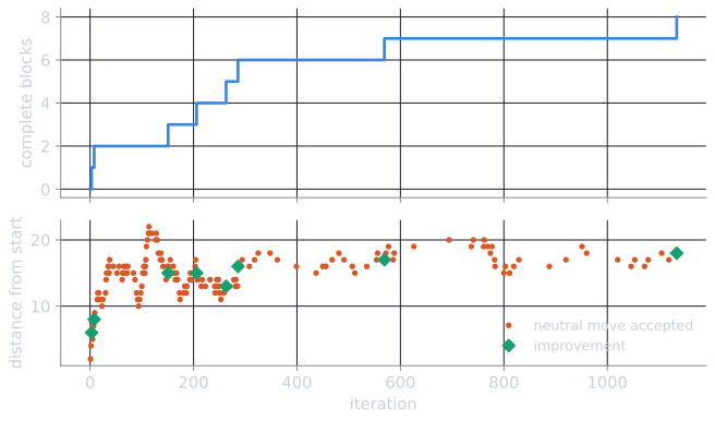
The flat stretches in the top panel are not idle time. The neutral moves carry the string across its plateau, and each improvement happens when a drifting incomplete block happens to complete. An algorithm that accepted only strict improvements would have to complete each block from wherever its bits happened to be, flipping all of the missing bits in one mutation, which is far less likely when two or three are missing.
Ruggedness and epistasis
A fitness landscape is rugged when neighboring points can have very different fitness, so that the value at one point says little about the values next to it. Weinberger (1990) proposed measuring this with the autocorrelation of fitness along a random walk: on a smooth fitness landscape, fitness values a few steps apart are still strongly correlated, and on a rugged one the correlation dies off quickly.
Ruggedness usually comes from epistasis, the biological term for interaction between genes, where the effect of one gene depends on the values of others. Without epistasis, every bit can be optimized separately, as in OneMax. Kauffman's NK model makes the amount of interaction a parameter (Kauffman and Levin, 1987; Kauffman and Weinberger, 1989). A string has $N$ binary loci. The fitness contribution $f_i$ of locus $i$ depends on its own value and the values of $K$ other loci, and each of the $2^{K+1}$ possible combinations is assigned an independent random number drawn uniformly from $[0, 1]$. Total fitness is the mean:
$$F(x) = \frac{1}{N} \sum_{i=1}^{N} f_i\bigl(x_i, x_{i_1}, \dots, x_{i_K}\bigr).$$
With $K = 0$ each locus contributes independently, so setting every bit to its better value gives a single optimum, and every other point has an improving neighbor. With $K = N - 1$ every contribution depends on the whole string, so changing one bit draws fresh random values for every term, and fitness values at neighboring points are effectively unrelated. For such an uncorrelated fitness landscape on the hypercube, a point is a local optimum when it is the best of itself and its $N$ neighbors, $N + 1$ independent values, which happens with probability $1/(N+1)$. The expected number of local optima is therefore $2^N / (N + 1)$, which for $N = 16$ is about 3,855, out of 65,536 points. Between the two extremes, $K$ tunes the fitness landscape from smooth to random.
How fast correlation decays with $K$. Weinberger's autocorrelation can be worked out for the NK model in a few lines. Take one step of a random walk: flip one bit, chosen uniformly. With the ring neighborhoods used here, that bit is read by exactly $K + 1$ of the $N$ contributions (its own and the $K$ loci before it), and the other $N - K - 1$ contributions do not change. Fitness is the mean of the contributions, each with the same variance $v$, so $\operatorname{Var}(F) = v/N$, and the covariance between the fitness before and after the step comes from the terms the two values share:
$$\rho(1) = \frac{\operatorname{cov}(F(x), F(x'))}{\operatorname{Var}(F)} \approx \frac{(N - K - 1)\, v / N^2}{v / N} = 1 - \frac{K + 1}{N}.$$
This assumes that each changed contribution takes a fresh, independent value. Inside one fixed instance it does not quite: a changed contribution moves to another entry of its own table of $M = 2^{K+1}$ random numbers, and two different entries of the same finite table are slightly negatively correlated, by $-1/(M - 1)$ on average, because they deviate from the same table mean. Including that term gives
$$\rho(1) \approx 1 - \frac{K + 1}{N} \cdot \frac{M}{M - 1}.$$
For $K = 0$ the correction is large: each contribution has only two values, and flipping its bit always swaps one for the other, so $\rho(1) = 1 - 2/N$. For $K \ge 4$ it is negligible. The script tools/experiments/evolution/landscape_structure.py measured both quantities exactly, over every edge of the hypercube, on 30 random instances for each $K$ from 0 to 15 with $N = 16$. The median measured $\rho(1)$ was 0.875 for $K = 0$ (corrected formula 0.875, uncorrected 0.938), 0.786 for $K = 2$ (0.786 and 0.813), 0.436 for $K = 8$ (0.436 and 0.438) and 0.000 for $K = 15$.
Along a longer walk the correlation at distance $d$ decays roughly as $\rho(1)^d$, since each step replaces another fraction of the contributions. On one instance with $K = 4$, a walk of 100,000 steps gave correlations of 0.675, 0.470 and 0.337 at distances 1, 2 and 3, against $\rho(1)^d$ = 0.677, 0.459 and 0.311. The measured values sit a little above the prediction because a walk sometimes flips the same bit back, undoing a step. For $K = 15$ this effect is the only correlation left: two steps return to the start with probability $1/16$, and the measured correlation at distance 2 was 0.069.
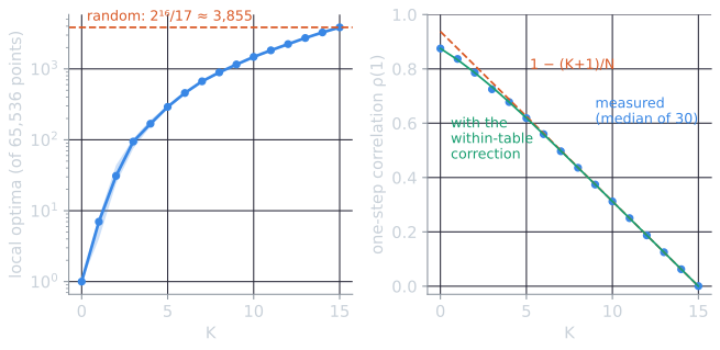
The local optima climb by more than three orders of magnitude, with medians of 1 at $K = 0$, 31 at $K = 2$, 168.5 at $K = 4$, 893 at $K = 8$ and 3,855 at $K = 15$, out of 65,536 points. Instances vary, most at small $K$: the single instance with $K = 2$ in the experiment below has 64 local optima, above the interquartile range of 24 to 44 for that $K$, while its instance with $K = 4$ has 173, inside the range of 155 to 191.
The demo's default instance, with $N = 10$ and $K = 2$, has 8 local optima among its 1,024 points and a fitness-distance correlation of $-0.354$, and steepest ascent from a uniformly random start reaches its global optimum 29.1% of the time; at $K = 0$ the same seed gives one optimum, reached from every start, and at $K = 9$ it gives 101 local optima and a success rate of 4.4% (script tools/experiments/evolution/nk_demo_check.py, which reproduces the demo's generator).
Deception
Deception, a notion from the theory of genetic algorithms developed by Goldberg and his colleagues, describes problems in which the information a genetic algorithm gathers about short building blocks points away from the optimum (see the schema theorem). Trap functions are the standard examples. They depend only on the number of ones $\lvert x \rvert$, rise steadily toward one end of the space, and place the global optimum at the other end. Deb and Goldberg (1993) analyzed which trap functions are deceptive in this sense. The Trap function of the introduction is the extreme case, credited by Droste, Jansen, and Wegener (2002) to Ackley (1987):
$$\mathrm{Trap}(x) = \lvert x \rvert + (n + 1) \prod_{i=1}^{n} (1 - x_i).$$
The product is 1 only for the all-zeros string. Every other string improves by gaining a one, so an improving search is led to the all-ones string, and from there the only improving move is to flip all $n$ bits at once. With bit-flip probability $1/n$, that happens with probability $n^{-n}$ per step. Droste, Jansen, and Wegener (2002) proved that the expected optimization time of the (1+1)-EA on Trap is $\Theta(n^n)$. For $n = 20$, $n^{-n}$ is about $9.5 \times 10^{-27}$.
With $n = 4$ the whole fitness landscape fits in a picture. Every string with $k \ge 1$ ones scores $k$, and 0000 scores $n + 1 = 5$.
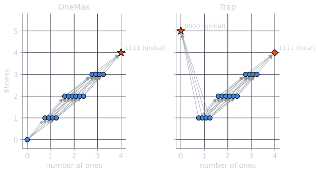
The picture shows how small the global optimum's basin is. Under steepest ascent, the climber moves to the best neighbor. From a string with a single one, the best neighbor is 0000 (fitness 5 against 2), so those four strings and 0000 itself form the basin of the global optimum: 5 of the 16 points. Every string with two or more ones climbs to 1111. For $n = 20$ the same reasoning gives a basin of 21 points out of $2^{20} = 1{,}048{,}576$, and a random start lands in it with probability about $2 \times 10^{-5}$.
Deception is a property of a fitness function together with a search process, not of the function alone. Trap is perfectly easy for an algorithm whose first guess is the all-zeros string, and for the complement operator above.
Fitness-distance correlation
Is there a number that predicts hardness? Jones and Forrest (1995) proposed fitness-distance correlation (FDC): the correlation coefficient between the fitness of a point and its distance to the nearest global optimum. Given fitness values $F$ and distances $D$ over a sample of points,
$$r = \frac{\operatorname{cov}(F, D)}{\sigma_F \, \sigma_D}.$$
For a maximization problem, fitness that rises as the distance to the optimum falls gives a negative $r$, and an improving search is led toward the optimum. A positive $r$ means that fitter points tend to lie farther away, so improvement leads the search astray. Jones and Forrest proposed rough bands: $r \le -0.15$ for straightforward problems, $r \ge 0.15$ for misleading ones, and the band in between, where the correlation says little, for difficult ones. On the problems they tested, FDC classified easy deceptive problems as easy and hard non-deceptive problems as hard, and it predicted when Gray coding outperformed binary coding.
Computing it by hand for a small case shows what the number measures. For OneMax on $n$ bits, a string with $k$ ones has fitness $k$ and distance $n - k$ to the all-ones optimum, so fitness is an exact decreasing linear function of distance and $r = -1$. For Trap, fitness equals distance everywhere except at the optimum itself, which is one point in $2^n$, so $r$ is just below $+1$. Every other function falls between these, and the exact values over all $2^{16}$ points for $n = 16$ are (script tools/experiments/evolution/landscape_structure.py, rounded to three decimals):
| Function ($n = 16$) | FDC |
|---|---|
| OneMax | −1.000 |
| Blocks of 4 (complete blocks of ones) | −0.516 |
| LeadingOnes (ones before the first zero) | −0.354 |
| NK, $K = 0$ | −0.723 |
| NK, $K = 2$ | −0.403 |
| NK, $K = 8$ | −0.046 |
| NK, $K = 15$ | −0.003 |
| Trap | +0.999 |
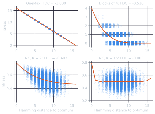
The table also shows that FDC is a statistic, not a verdict. LeadingOnes has a weaker correlation than the block function, yet the $(1+1)$-EA solves it reliably in $\Theta(n^2)$ expected time (Droste, Jansen, and Wegener, 2002), because every non-optimal string has an improving one-bit neighbor. The correlation is weak because many points far from the optimum have a fitness of 0 or 1, not because the search is led astray.
FDC has clear limits. It needs the global optimum, so it is a tool for studying benchmark problems, not for diagnosing a new one. It compresses an entire fitness landscape into one linear statistic, and constructed problems exist on which it gives the wrong answer. Tomassini, Vanneschi, Collard, and Clergue (2005) found it a useful indicator for genetic programming problems in nearly all their cases, and also built an artificial problem on which it gives contradictory indications. The distance in the formula must also match the operator. Hamming distance suits bit-flip mutation and says nothing about a complement operator.
Experiment: one algorithm, three kinds of problem
The (1+1)-EA is the simplest evolutionary algorithm: a population of one parent and one child. It starts from a random bitstring $x$, creates a child $y$ by flipping each bit independently with probability $1/n$, and replaces $x$ by $y$ if $f(y) \ge f(x)$. Accepting equal fitness lets it drift across plateaus. Each problem below gets 30 seeded runs. FDC is computed exactly over the whole search space, using Hamming distance to the global optimum.
OneMax. Here the fitness landscape is as smooth as possible, and $f(x) = n - d(x)$, where $d$ is the distance to the all-ones optimum, so FDC is exactly $-1$. A standard argument bounds the run time. With $i$ zeros left, one way to improve is to flip exactly one of those $i$ bits and nothing else, which has probability $i \cdot \frac{1}{n} (1 - \frac{1}{n})^{n-1} \ge \frac{i}{en}$. The expected wait at that level is at most $en/i$ iterations, and summing over $i = 1, \dots, n$ gives at most $e n H_n \approx e n \ln n$, where $H_n$ is the $n$-th harmonic number. Droste, Jansen, and Wegener (2002) proved that every linear function, OneMax included, is optimized in expected time $O(n \ln n)$. The precise constant took longer: Hwang, Panholzer, Rolin, Tsai, and Chen (2018) give the expected number of iterations as
$$e n \ln n - 1.89254\, n + \tfrac{e}{2} \ln n + 0.59790 + O\!\left(\tfrac{\ln n}{n}\right).$$
| $n$ | Median iterations (IQR) | Mean | $e n \ln n$ | Hwang et al. |
|---|---|---|---|---|
| 25 | 154 (132 to 201) | 170 | 219 | 176 |
| 50 | 386 (335 to 466) | 424 | 532 | 443 |
| 100 | 1,074 (928 to 1,312) | 1,124 | 1,252 | 1,069 |
| 200 | 2,317 (2,061 to 2,774) | 2,557 | 2,880 | 2,510 |
The sample means are within about one standard error of the expansion, and well below $e n \ln n$, whose linear correction is still large at these sizes. The medians sit below the means because the distribution of run times has a long right tail: most of the time is spent at the end, waiting for the last few zeros to be hit.
Trap, with $n = 20$ and a budget of 100,000 evaluations: 0 of 30 runs found the optimum, and all 30 ended at the all-ones string. FDC is $+1.000$ to three decimals, since Trap equals the distance to the optimum everywhere except at the optimum itself, one point in $2^{20}$. The prediction of FDC and the behavior of the algorithm agree.
NK model, with $N = 16$ and $K$ other loci taken to be the next $K$ positions around a ring. One random instance per $K$, enumerated in full (65,536 points) to find its global optimum and count its local optima under single-bit flips. Each run had a budget of 20,000 evaluations.
| $K$ | Local optima | FDC | Runs that found the optimum | Median evaluations when found (IQR) |
|---|---|---|---|---|
| 0 | 1 | −0.723 | 30 / 30 | 87 (68 to 127) |
| 2 | 64 | −0.403 | 26 / 30 | 634 (406 to 1,072) |
| 4 | 173 | −0.156 | 10 / 30 | 762 (546 to 968) |
| 8 | 931 | −0.046 | 2 / 30 | 5,350 (2,771 to 7,930) |
| 15 | 3,813 | −0.003 | 0 / 30 | none |
As $K$ grows, local optima multiply, the correlation between fitness and distance to the optimum fades to nothing, and success falls from 30 runs to none. At $K = 15$ the count of 3,813 local optima is close to the $2^{16}/17 \approx 3{,}855$ expected for an uncorrelated fitness landscape. The (1+1)-EA is not a pure hill climber, since it occasionally flips several bits at once, which is how most of the successful runs at $K = 2$, 4, and 8 got past a local optimum on the way. These are single instances of each problem, so the exact counts would shift with a different random draw, but the trend is the one Kauffman's model is designed to produce. The script is tools/experiments/evolution/landscapes.py in the site repository.
Limits of the picture
The fitness landscape is a useful model of a single-point search with one operator. It is less faithful for the algorithms the rest of this course studies. A population with crossover moves in ways that depend on the whole population, not on one point's neighbors. In high dimensions, intuitions from two-dimensional pictures mislead: a point that looks trapped on a map may have many escape routes through dimensions the picture cannot show, which is the same caution Wright gave about his own diagram. When fitness depends on other evolving individuals, as in competitive coevolution, the fitness landscape itself changes as the search moves, and peaks stop being fixed targets (Red Queen dynamics). Finally, no single feature determines difficulty. FDC, ruggedness, and counts of local optima are all summaries, and each has counterexamples.
The fitness landscape also frames the question taken up in the No Free Lunch theorems: averaged over every possible arrangement of fitness values, every search algorithm performs equally. Algorithms succeed on real problems because those problems have structure, such as smoothness, low epistasis, or a strong correlation between fitness and distance to the optimum, that the algorithm's operators can exploit.
References
- Ackley, D. H. (1987). A Connectionist Machine for Genetic Hillclimbing. Kluwer Academic Publishers.
- Deb, K., and Goldberg, D. E. (1993). Analyzing deception in trap functions. In L. D. Whitley (Ed.), Foundations of Genetic Algorithms 2, 93–108. Morgan Kaufmann.
- Droste, S., Jansen, T., and Wegener, I. (2002). On the analysis of the (1+1) evolutionary algorithm. Theoretical Computer Science, 276(1–2), 51–81.
- Eiben, A. E., and Smith, J. E. (2015). Introduction to Evolutionary Computing, 2nd ed., chapter 2. Springer.
- Hwang, H.-K., Panholzer, A., Rolin, N., Tsai, T.-H., and Chen, W.-M. (2018). Probabilistic analysis of the (1+1)-evolutionary algorithm. Evolutionary Computation, 26(2), 299–345.
- Jones, T. (1995). Evolutionary Algorithms, Fitness Landscapes and Search. PhD thesis, University of New Mexico.
- Jones, T., and Forrest, S. (1995). Fitness distance correlation as a measure of problem difficulty for genetic algorithms. In Proceedings of the Sixth International Conference on Genetic Algorithms (ICGA 1995), 184–192. Morgan Kaufmann.
- Kauffman, S., and Levin, S. (1987). Towards a general theory of adaptive walks on rugged landscapes. Journal of Theoretical Biology, 128(1), 11–45.
- Kauffman, S. A., and Weinberger, E. D. (1989). The NK model of rugged fitness landscapes and its application to maturation of the immune response. Journal of Theoretical Biology, 141(2), 211–245.
- Skipper, R. A., Jr. (2004). The heuristic role of Sewall Wright's 1932 adaptive landscape diagram. Philosophy of Science, 71(5), 1176–1188.
- Tomassini, M., Vanneschi, L., Collard, P., and Clergue, M. (2005). A study of fitness distance correlation as a difficulty measure in genetic programming. Evolutionary Computation, 13(2), 213–239.
- Weinberger, E. (1990). Correlated and uncorrelated fitness landscapes and how to tell the difference. Biological Cybernetics, 63(5), 325–336.
- Wright, S. (1932). The roles of mutation, inbreeding, crossbreeding and selection in evolution. In Proceedings of the Sixth International Congress of Genetics, 1, 356–366.