Take a search space of eight points, the bitstrings of length three, and suppose each point can score 0, 1, or 2. There are $3^8 = 6{,}561$ possible fitness functions. Now compare two search algorithms. The first evaluates the points in a fixed order, $000, 001, 010, \dots, 111$, whatever it sees. The second is a hill climber: it starts at $111$, and at each step evaluates an unvisited neighbor (one bit flip away) of the best point found so far, or, if that point has no unvisited neighbor, the first unvisited point in the fixed order. Run both on all 6,561 functions and record, for each, the best value found after $m$ evaluations. The hill climber uses everything it learns, and the fixed order uses nothing. Yet the two histograms are identical for every $m$, count for count.
This is an instance of the No Free Lunch (NFL) theorem for optimization of Wolpert and Macready (1997). The theorem is precise and its proof is short. Its interpretation has been argued over ever since. This article states the theorem carefully, gives the intuition for why it holds, presents the sharpened version that says exactly which sets of problems it applies to, and then sets out what it implies for evolutionary algorithms and what it does not.
The setting
The theorem concerns a deliberately abstract model of black-box optimization:
- A finite search space $X$ and a finite set of values $Y$, totally ordered. A problem is a function $f : X \to Y$, and $\mathcal{F} = Y^X$ is the set of all such functions. The example has $\lvert X \rvert = 8$, $\lvert Y \rvert = 3$, and $\lvert \mathcal{F} \rvert = 6{,}561$.
- A search algorithm chooses the next point to evaluate from the history of points evaluated so far and their values. It learns about $f$ only by evaluating it. The algorithm is non-revisiting: it never evaluates the same point twice.
- After $m$ evaluations the algorithm has produced a sequence of values $d^y_m = \bigl(f(x_1), \dots, f(x_m)\bigr)$. A performance measure is any function of this sequence, such as the best value seen, or the number of evaluations until the best value was first seen.
The restriction to non-revisiting algorithms is less limiting than it looks. A revisit gains no information, so an algorithm that revisits can be compared fairly by counting only its distinct evaluations, which is what Wolpert and Macready do. Real evolutionary algorithms do revisit points, and an evaluation spent on a duplicate is simply wasted.
The theorem
For any two algorithms $a_1$ and $a_2$, any number of evaluations $m$, and any sequence of values $d^y_m$,
$$\sum_{f \in \mathcal{F}} P(d^y_m \mid f, m, a_1) = \sum_{f \in \mathcal{F}} P(d^y_m \mid f, m, a_2).$$
This is Theorem 1 of Wolpert and Macready (1997). They define algorithms as deterministic and show that the result extends to stochastic ones. For a deterministic algorithm, $P(d^y_m \mid f, m, a)$ is 1 for the one sequence the algorithm produces on $f$ and 0 otherwise, so the theorem says that the two algorithms produce exactly the same multiset of value sequences across all functions. Since any performance measure is a function of the sequence, every performance measure has the same distribution across all functions, and the same average.
The reason is easiest to see probabilistically. Choosing $f$ uniformly from $\mathcal{F}$ is the same as choosing each value $f(x)$ independently and uniformly from $Y$. Whatever the algorithm has seen so far, the values at the points it has not yet visited are still independent and uniform. So whichever unvisited point it picks next, the value it observes is a fresh uniform draw. Every algorithm, however clever, observes a sequence of independent uniform values. Picking points at random without replacement does exactly as well.
The whole theorem on three points
The smallest interesting case can be written out completely. Let $X = \{p, q, r\}$ and $Y = \{0, 1\}$, so there are $2^3 = 8$ functions. Algorithm F evaluates $p$, $q$, $r$ in that order. Algorithm A is adaptive: it evaluates $q$ first, then $r$ if $f(q) = 1$ and $p$ otherwise, and then the remaining point. The table lists, for every function, the points each algorithm visits and the sequence of values it observes (script tools/experiments/evolution/nfl_small.py).
| $f(p)\,f(q)\,f(r)$ | F visits | F sees | A visits | A sees |
|---|---|---|---|---|
| 000 | p q r | 000 | q p r | 000 |
| 001 | p q r | 001 | q p r | 001 |
| 010 | p q r | 010 | q r p | 100 |
| 011 | p q r | 011 | q r p | 110 |
| 100 | p q r | 100 | q p r | 010 |
| 101 | p q r | 101 | q p r | 011 |
| 110 | p q r | 110 | q r p | 101 |
| 111 | p q r | 111 | q r p | 111 |
On five of the eight functions the two algorithms see different sequences, but each column of observed sequences contains each of the eight possible sequences exactly once. So any performance measure, computed from the sequences, has the same distribution for both: for example, the best of the first two values is 1 on 6 of the 8 functions for both algorithms, and the best of the first value alone on 4.
The table is an instance of a counting argument that proves the theorem for deterministic algorithms in general.
- Fix a deterministic, non-revisiting algorithm and run it on $f$ until it has evaluated every point. It observes a sequence of $\lvert X \rvert$ values.
- The sequence determines $f$. The algorithm's first point is fixed; the first value determines its second point; the first two values determine its third; and so on. Replaying the algorithm against the sequence recovers which point received each value, which is all of $f$.
- So different functions give different sequences. There are $\lvert Y \rvert^{\lvert X \rvert}$ functions and $\lvert Y \rvert^{\lvert X \rvert}$ possible sequences, so the map from functions to sequences is a bijection: as $f$ runs over all functions, the algorithm sees every sequence exactly once.
- Therefore each possible sequence of $m$ first values occurs for exactly $\lvert Y \rvert^{\lvert X \rvert - m}$ functions, for every algorithm.
The algorithm decides only which function produces which sequence, not which sequences occur. For the two algorithms of the introduction, and for a hill descender that follows the worst point seen, each of the 6,561 functions on three bits gives a distinct sequence, as step 3 requires. Step 4 gives the first table below directly: the best of $m$ values is at most $v$ exactly when all $m$ values are at most $v$, which happens for a fraction $\bigl((v+1)/\lvert Y \rvert\bigr)^m$ of the functions.
The enumeration confirms this for the two algorithms of the introduction. The table gives, for each $m$, how many of the 6,561 functions leave each algorithm with best value 0, 1, or 2, and the mean.
| $m$ | Fixed order: 0 / 1 / 2 | Hill climber: 0 / 1 / 2 | Mean best |
|---|---|---|---|
| 1 | 2,187 / 2,187 / 2,187 | 2,187 / 2,187 / 2,187 | 1.000 |
| 2 | 729 / 2,187 / 3,645 | 729 / 2,187 / 3,645 | 1.444 |
| 4 | 81 / 1,215 / 5,265 | 81 / 1,215 / 5,265 | 1.790 |
| 8 | 1 / 255 / 6,305 | 1 / 255 / 6,305 | 1.961 |
The counts can be checked by hand. The best of $m$ values is 0 only if all $m$ are 0, which happens for $3^{8-m}$ functions (729 for $m = 2$). It is at most 1 for $2^m \cdot 3^{8-m}$ functions, so it is exactly 1 for $2^m 3^{8-m} - 3^{8-m}$ of them (2,187 for $m = 2$). Both algorithms also need, on average, 2.647 evaluations to first see the function's maximum value, with identical histograms.
Sets closed under permutation
The theorem averages over all functions. A natural question is whether it holds for smaller sets, and Schumacher, Vose, and Whitley (2001) answered it exactly. A permutation $\sigma$ of $X$ shuffles the points, and $f \circ \sigma$ is the function that takes the same values at the shuffled positions. A set of functions $F$ is closed under permutation (c.u.p.) if $f \circ \sigma$ is in $F$ for every $f \in F$ and every permutation $\sigma$. The sharpened NFL theorem states that all algorithms have the same performance distribution averaged uniformly over $F$ if and only if $F$ is closed under permutation.
Closure under permutation has a simple description. Two functions are permutations of each other exactly when they take each value the same number of times, that is, when they have the same histogram of values. A set is c.u.p. exactly when it is a union of whole histogram classes (Igel and Toussaint, 2003). For example, the 168 functions on the three-bit space that take the value 2 once, 1 twice, and 0 five times form one class. On that set, the fixed order and the hill climber again give identical histograms. Both need 4.5 evaluations on average to find the single point with value 2, and the number needed is spread evenly over 1 to 8, 21 functions each. That average matches a general formula Igel and Toussaint (2004) summarize: averaged over all functions with $k$ optimal points out of $\lvert X \rvert$, any non-revisiting algorithm needs $(\lvert X \rvert + 1)/(k + 1)$ evaluations to find one, here $9/2$.
The formula has a short derivation. Write $n = \lvert X \rvert$. Averaged over all placements of the $k$ optimal points, the order in which an algorithm visits points does not matter: until it finds an optimum it has seen only non-optimal values, and the optima are equally likely to be at any point it has not yet visited. So it may as well use a fixed order, and the $k$ optimal points sit at uniformly random positions in it. They divide the $n - k$ other points into $k + 1$ gaps: before the first optimum, between consecutive optima, and after the last. By symmetry the gaps have equal expected size, $(n - k)/(k + 1)$. The algorithm evaluates the whole first gap and then the first optimum, so it needs $(n - k)/(k + 1) + 1 = (n + 1)/(k + 1)$ evaluations on average. Enumerating all placements for $n = 8$ gives exactly $9/2$, $3$ and $9/4$ for $k = 1$, 2 and 3.
Igel and Toussaint (2004) extended the result to non-uniform distributions over functions. All algorithms perform equally, for every performance measure, if and only if functions with the same histogram are equally likely. The condition is again about symmetry: no arrangement of a given set of values may be favored over another.
What the theorems imply
The theorems rule out a certain kind of claim. A statement such as "algorithm $A$ is better than algorithm $B$ on average over all problems" is false for every pair of algorithms. It is also false over any c.u.p. set with uniform weights. Any gain an algorithm shows on some functions is paid for exactly on the others. Wolpert and Macready drew the practical conclusion that effective optimization depends on a match between the algorithm and the distribution of problems it is run on, so a claim that one algorithm is better than another means something only relative to a class of problems. Evolutionary algorithms are not exempt. Averaged over all functions on a finite space, a genetic algorithm does no better than random search without replacement, and no worse.
What the theorems do not imply
The theorems do not say that all algorithms are equally good on the problems people actually solve, because those problems are not a c.u.p. set chosen uniformly.
C.u.p. sets are rare. A set of functions is c.u.p. only if it is a union of histogram classes. The number of histogram classes is $\binom{\lvert X \rvert + \lvert Y \rvert - 1}{\lvert X \rvert}$, so the number of non-empty c.u.p. sets is $2^{\binom{\lvert X \rvert + \lvert Y \rvert - 1}{\lvert X \rvert}} - 1$, out of $2^{\lvert Y \rvert^{\lvert X \rvert}} - 1$ non-empty sets in all (Igel and Toussaint, 2003). For the three-bit example there are $\binom{10}{8} = 45$ classes, so $2^{45} - 1 \approx 3.5 \times 10^{13}$ of the $2^{6561} - 1$ sets are c.u.p., a fraction of about $10^{-1962}$. A set of problems chosen without the symmetry in mind will almost never satisfy the theorem's precondition.
Structure breaks the symmetry. The properties that make problems tractable are defined by neighborhoods, and a non-trivial neighborhood relation is not preserved by arbitrary permutations of the points. Igel and Toussaint (2003) showed that if every function in a set is limited to less than the maximum possible steepness between neighbors, or to fewer than the maximum possible number of local minima, the set is not c.u.p. A problem class described as "smooth" or "not maximally rugged" therefore lies outside the theorem, and in the terms of fitness landscapes, that is most problem classes anyone cares about.
The enumeration shows the effect on a small scale. Restrict the three-bit example to the 743 smooth functions, those in which neighboring points differ in value by at most 1. This set is not c.u.p., and the two algorithms now differ:
| $m$ | Fixed order: mean best | Hill climber: mean best |
|---|---|---|
| 2 | 1.280 | 1.280 |
| 3 | 1.420 | 1.444 |
| 4 | 1.503 | 1.542 |
| 5 | 1.561 | 1.594 |
| 8 | 1.654 | 1.654 |
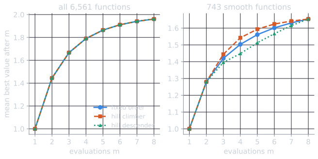
The hill climber needs 2.370 evaluations on average to find a maximum, against 2.501 for the fixed order. The advantage is small, as might be expected on eight points, and it is not uniform: after four evaluations the hill climber is stuck at 0 on 17 functions, against 16 for the fixed order. But the equality that held for every $m$ and every count is gone, because the hill climber's assumption, that good points have good neighbors, is built into the set of problems. The script is tools/experiments/evolution/nfl_check.py in the site repository.
Structure helps only an algorithm that matches it. Wolpert and Macready (1997) stress the other side of this point. The mere existence of structure in a problem class does not justify choosing a particular algorithm; the structure has to be known and reflected in the algorithm. On the smooth functions above, a hill descender, which follows the worst point seen instead of the best, needs 2.678 evaluations on average to find a maximum, worse than the fixed order's 2.501, for exactly the reason the hill climber does better. Over all 6,561 functions it too ties with the other two.
Averages are not guarantees about a particular problem. The theorems concern averages over a set of functions. They say nothing about which algorithm is better on a given function, and nothing about problems drawn from a distribution concentrated on structured functions, which is the situation the fitness landscape experiments describe.
Continuous domains
The original theorem needs $X$ and $Y$ to be finite, so that a uniform distribution over all functions makes sense. A continuous search space, such as the real vectors that evolution strategies and CMA-ES optimize, has no uniform distribution over all functions, and the question becomes what a "random fitness function" should mean. Auger and Teytaud (2010) formalized random fitness functions as random fields and showed that, in continuous domains, NFL does not hold: free lunches exist, and some algorithms are better than others averaged over such distributions. They also used the same framework to derive optimal optimization algorithms for a given distribution of fitness functions and a given budget of evaluations.
A floating-point search space is finite, so the original theorem does apply to it formally. That does not rescue the strong reading of NFL. The theorem would require averaging uniformly over all functions on the floating-point grid, nearly all of which look like noise at every scale, while continuous optimizers are designed for, and tested on, functions whose values vary smoothly with their arguments.
Summary
The No Free Lunch theorems are correct and their conditions are exact: averaged uniformly over all functions on a finite space, or over any set closed under permutation, every non-revisiting search algorithm performs the same. They are best read as a statement about where an algorithm's power comes from (Eiben and Smith, 2015, ch. 16). No algorithm is good in general. An algorithm is good on a class of problems when its operators and selection exploit structure that the class actually has, the subject of fitness landscapes and of the course's other topics.
References
- Auger, A., and Teytaud, O. (2010). Continuous lunches are free plus the design of optimal optimization algorithms. Algorithmica, 57(1), 121–146.
- Eiben, A. E., and Smith, J. E. (2015). Introduction to Evolutionary Computing, 2nd ed., chapter 16. Springer.
- Igel, C., and Toussaint, M. (2003). On classes of functions for which No Free Lunch results hold. Information Processing Letters, 86(6), 317–321.
- Igel, C., and Toussaint, M. (2004). A No-Free-Lunch theorem for non-uniform distributions of target functions. Journal of Mathematical Modelling and Algorithms, 3(4), 313–322.
- Schumacher, C., Vose, M. D., and Whitley, L. D. (2001). The No Free Lunch and problem description length. In Proceedings of the Genetic and Evolutionary Computation Conference (GECCO 2001), 565–570. Morgan Kaufmann.
- Wolpert, D. H., and Macready, W. G. (1997). No free lunch theorems for optimization. IEEE Transactions on Evolutionary Computation, 1(1), 67–82.