Suppose a network must look at an 11 by 11 grid of light sensors and mark, on an 11 by 11 grid of outputs, where the larger of two objects lies. Connecting every sensor to every output takes $121 \times 121 = 14{,}641$ weights. NEAT and the weight-evolving methods before it encode networks directly: each connection is a gene, so the genome for this task would have 14,641 weights to tune, one at a time. Yet the right answer has an obvious structure. Every sensor should do the same thing, excite the outputs near its own position, and a rule that is true for one sensor is true for all of them. A direct encoding cannot say "the same rule everywhere"; it has to discover the rule 121 times over.
Biology avoids this problem. The human genome holds far fewer genes than the brain has connections, so the genome cannot list connections one by one. It describes instead a process that produces them, and the regularities of the body, its symmetry and its repeated parts, come from reusing the same genetic information in many places. An indirect (or generative) encoding imitates this: the genome is a compact description that is expanded into the phenotype, and one gene can affect many parts of it.
This article describes one line of indirect encodings developed by Kenneth Stanley and his colleagues. Compositional pattern-producing networks (CPPNs) represent a pattern as a composition of simple functions of position (Stanley, 2007). HyperNEAT reads a CPPN as the connectivity pattern of a neural network whose neurons have positions in space (Stanley, D'Ambrosio, and Gauci, 2009). Both are evolved with NEAT, and both depend on what NEAT contributes: growth from small networks, crossover by historical markings, and speciation.
Patterns as compositions of functions
Stanley (2007) starts from developmental biology. In an embryo, cells learn where they are from chemical gradients, and later structures are laid out relative to earlier ones. His observation is that the result of this process can be described without simulating it. Let $x$ be the left-right coordinate. A gradient that peaks at the midline and falls off on both sides, the basis of bilateral symmetry, is simply a symmetric function of $x$, such as a Gaussian or $|x|$. A row of segments along the head-to-tail axis $y$ is a periodic function such as $\sin(y)$. Feed the output of a symmetric function into a periodic one and the result is two sets of segments with opposite polarity, mirrored about the midline. Each composition creates a new coordinate frame that later functions can build on, so the order of composition plays the role of developmental time (Stanley, 2007, §3.2).
A composition of many functions is naturally drawn as a graph: coordinates enter at the inputs, each node applies a function to the weighted sum of its inputs, and the output is the value of the pattern at that point. That graph is a neural network in all but name, with one difference: an ordinary artificial neural network generally uses sigmoids (and sometimes Gaussians) at its nodes, while the composition graph may use any of a set of canonical functions at each node. Stanley named it a compositional pattern-producing network to avoid implying that it models a brain. To draw a two-dimensional image, the CPPN is queried once per pixel with that pixel's coordinates, and the output sets its intensity. Each pixel is computed independently of every other, so there is no simulated growth and no interaction between neighbouring cells; the cost is one network activation per point (Stanley, 2007, §3.2 and §3.5).
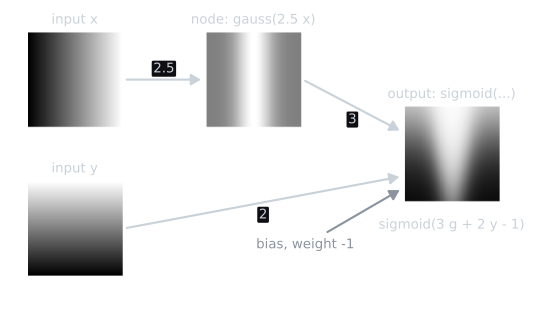
Querying one pixel by hand shows what "compose" means. With $\mathrm{gauss}(z) = e^{-z^2}$ and the signed sigmoid $\mathrm{sigmoid}(z) = 2/(1 + e^{-z}) - 1$, the CPPN in the figure computes $\mathrm{sigmoid}(3\,\mathrm{gauss}(2.5x) + 2y - 1)$. At the point $(0.5, 0.5)$ the hidden node receives $2.5 \times 0.5 = 1.25$ and outputs $e^{-1.5625} = 0.2096$; the output node's sum is $3 \times 0.2096 + 2 \times 0.5 - 1 = 0.6288$, and the pixel's value is $\mathrm{sigmoid}(0.6288) = 0.3045$. At the mirror point $(-0.5, 0.5)$ the hidden node receives $-1.25$, and because the Gaussian is even it outputs the same 0.2096, so every later value is identical. At the centre the Gaussian peaks at 1 and the pixel is $\mathrm{sigmoid}(2) = 0.7616$. Nothing in the network says "be symmetric"; the symmetry is a consequence of an even function sitting between $x$ and everything downstream of it. (Values from tools/experiments/evolution/cppn_worked.py, rounded to four decimals.)
The choice of activation functions is what gives CPPNs their bias toward natural-looking regularity. Stanley (2007, §2.2) lists the regularities he wanted an encoding to produce, and each has a simple functional source:
| Regularity | Function that produces it |
|---|---|
| Symmetry | an even function of a coordinate: a Gaussian, $\lvert x \rvert$, or the distance $d$ from the centre |
| Repetition | a periodic function: $\sin$, or $y \bmod 1$ for repeated frames that are not themselves symmetric |
| Repetition with variation | a periodic function combined with a non-periodic one, so the copies differ by position |
| Imperfect symmetry | a symmetric function combined with an asymmetric gradient such as $x$ itself |
In the paper's main image experiments the CPPNs received $x$, $y$ and the distance $d$ from the centre as inputs. Including $d$ biases the patterns toward symmetry, but only radial symmetry; bilateral symmetry still has to be built from functions of $x$ (Stanley, 2007, Fig. 6).
Five hand-built CPPNs
The script tools/experiments/evolution/cppn_patterns.py renders five CPPNs written by hand, not evolved, at 96 by 96 pixels over $x, y \in [-1, 1]$ and saves them as grayscale images. It also measures two regularities directly on the pixel grid: the largest difference between a pixel and its mirror image across $x = 0$, and the largest difference between $f(x, y)$ and $f(x + p, y)$ for a stated period $p$. Here $\mathrm{gauss}(z) = e^{-z^2}$ and the sigmoid is the signed version $2/(1 + e^{-z}) - 1$.
| CPPN | What the image shows | Mirror error | Period error |
|---|---|---|---|
| $\mathrm{sigmoid}(3\,\mathrm{gauss}(2.5x) + 2y - 1)$ | a bright vertical band at the centre, fading toward the bottom | 0.000 | |
| $\sin(4\pi x)\,\mathrm{gauss}(2y)$ | four light and four dark vertical bars across the middle | 1.999 | 0.000 ($p = 0.5$) |
| $\sin(6\pi\lvert x \rvert)\,\mathrm{sigmoid}(4y)$ | stripes that mirror each other about the centre line | 0.000 | |
| $\sin(4\pi x)\,\mathrm{gauss}(2y - x)$ | the same bump repeated four times, each copy higher than the last | 1.959 | 0.411 ($p = 0.5$) |
| $\sin(5\pi d)\,\mathrm{gauss}(1.5d)$ | concentric rings fading outward | 0.000 |
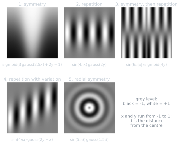
Only the first of the five is a CPPN in the strict sense of Stanley's (2007) formulation, in which every node applies its function to a weighted sum of its inputs. The other four multiply two functions, a step outside that formulation; they are written as formulas so that each isolates one regularity, and an evolved CPPN would have to produce a similar effect by composition instead.
The first image is exactly symmetric because $x$ enters only through a Gaussian. The second repeats exactly with period 0.5 and is not symmetric (its mirror error is the full range of the pattern), because the sine is odd. The third composes a symmetric function, $\lvert x \rvert$, into a periodic one, Stanley's example of two sets of segments with opposite polarity. The fourth shows repetition with variation: the sine places four bumps, and the Gaussian of $2y - x$ moves each one vertically by an amount that depends on $x$. The brightest pixel in the column of each crest lies at $y = -0.432$, $-0.179$, $0.053$ and $0.305$, so the motif repeats but no two copies are identical. The fifth is symmetric about both axes because it depends only on $d$. Small formulas, a few nodes each, give patterns whose regularity is exact, and the regularity follows from the functions chosen, not from anything pixel-by-pixel.
Two experiments with the demo make the article's table concrete. Starting from preset 1, give the hidden node H1 any weight from $y$: the band tilts, and the mirror error, 0.000 before, becomes positive, because $x$ now reaches the output through a sum that is no longer even in $x$. Or change H1's function from gauss to linear: the band becomes a left-to-right ramp and the symmetry disappears for the same reason. Symmetry survives any edit that keeps $x$ entering only through even functions: changing the weight from $x$ into H1, or the weights of the output node's existing connections from H1, $y$ and the bias, reshapes the pattern but leaves the mirror error at 0. For this CPPN, then, a mutation of an existing weight can vary the pattern but cannot break its symmetry; only a new connection, such as one from $y$ into the Gaussian node or one from $x$ straight to the output, or a change of the hidden node's function, can.
CPPN-NEAT and interactive evolution
Stanley (2007) evolved CPPNs with an extension of NEAT, CPPN-NEAT. Node genes gain a field for the activation function, and a new node created by mutation takes a random function from a canonical set, including Gaussian, sigmoid and periodic functions. The compatibility distance used for speciation gains a term counting how many activation functions differ between two genomes, so networks with different functions can fall into different species (Stanley, 2007, §3.4).
The experiments in that paper used interactive evolution: a person looks at the images of the current population and picks one or two parents for the next generation. Fitness is the person's judgement, so speciation was switched off; structural mutation still complexified the CPPNs over the generations. Stanley reports evolved images that elaborate on a symmetric theme, represent imperfect symmetry, and repeat a motif with variation (Stanley, 2007, §4.2 to §4.4).
Picbreeder turned this into a public website (Secretan et al., 2011). Visitors evolve images by selecting from a population of CPPN-generated pictures, publish the ones they like, and continue evolving images that others published, a step the paper calls branching. A single person can judge only so many generations before tiring, which limits how far interactive evolution can go; on Picbreeder one user's lineage can be picked up by another, so an image can be the product of selection by many people in turn. The paper discusses the strengths of the approach and its shortcomings.
HyperNEAT: a CPPN as a connectivity pattern
A CPPN that maps two coordinates to an intensity draws a picture. HyperNEAT makes it draw a network instead. Its key step is to give the CPPN the coordinates of two points and to read the output as the weight of a connection between them (Gauci and Stanley, 2007; Stanley, D'Ambrosio, and Gauci, 2009):
$$w = \mathrm{CPPN}(x_1, y_1, x_2, y_2),$$
where $(x_1, y_1)$ is the position of the source neuron and $(x_2, y_2)$ the position of the target. A four-input CPPN describes a pattern inside a four-dimensional hypercube, and each point of that hypercube is a possible connection, hence the name: hypercube-based NEAT.
The neurons themselves are not evolved. The experimenter places them in a geometric layout called the substrate, for instance a grid of input neurons in the plane and a grid of output neurons above it, with coordinates in $[-1, 1]$. To build a network, every potential connection on the substrate is queried in turn. By the convention of Gauci and Stanley (2007), a connection whose CPPN output has magnitude at most 0.2 is not expressed, and larger magnitudes are rescaled to between zero and a maximum weight of 3, keeping the sign. The CPPN is evolved with NEAT, and each CPPN is evaluated by building its substrate network and running that network on the task.
Because the weight is a function of the two neurons' positions, the geometry of the substrate becomes meaningful. A CPPN that computes a function of $x_1 - x_2$ gives every source neuron the same pattern of connections relative to its own position: a convolution-like, repeated motif, discovered once and expressed everywhere. A CPPN symmetric in $x_1$ gives mirror-image connections on the two sides of the substrate. The regularities of CPPN images become regularities of connectivity. This only helps if the experimenter's layout matches the geometry of the task, placing sensors where they are in the world, for example, and HyperNEAT's results depend on that choice.
One CPPN, several resolutions
The second part of cppn_patterns.py shows the mechanism on a one-dimensional substrate: a row of $n$ input neurons at $x_1 \in [-1, 1]$ and a row of $n$ output neurons at $x_2 \in [-1, 1]$, with the hand-built connective CPPN
$$w(x_1, x_2) = 1.4\,\mathrm{gauss}\big(2.5\,(x_1 - x_2)\big) - 0.4,$$
which excites outputs near each input and weakly inhibits distant ones. The threshold and rescaling of Gauci and Stanley (2007), implemented in the script as a linear map, turn a raw output $r$ into a weight
$$w = \begin{cases} 0 & \text{if } |r| \le 0.2, \\ \mathrm{sign}(r)\,\dfrac{|r| - 0.2}{1 - 0.2} \times 3 & \text{otherwise,} \end{cases}$$
so that raw outputs from 0.2 to 1 in magnitude map linearly onto weights from 0 to 3. Three queries into the output neuron at $x_2 = 0$, from cppn_worked.py:
| Source $x_1$ | $x_1 - x_2$ | $\mathrm{gauss}(2.5(x_1 - x_2))$ | Raw $r$ | Expressed weight |
|---|---|---|---|---|
| 0 | 0 | 1.0000 | 1.000 | $(1 - 0.2)/0.8 \times 3 = 3.000$ |
| $-0.5$ | $-0.5$ | 0.2096 | $-0.107$ | none ($\lvert r \rvert \le 0.2$) |
| $-1$ | $-1$ | 0.0019 | $-0.397$ | $-(0.397 - 0.2)/0.8 \times 3 = -0.740$ |
On five neurons per row, with coordinates $-1, -0.5, 0, 0.5, 1$, the raw outputs are 1 on the diagonal, $-0.107$ for neighbours 0.5 apart, $-0.397$ at distance 1 and $-0.400$ beyond. After the 0.2 threshold and rescaling, the diagonal weights are 3.000, neighbouring connections are not expressed (their magnitude is below 0.2), and the rest are $-0.740$ or $-0.750$. The resulting matrix is a band: the same rule in every row, shifted.
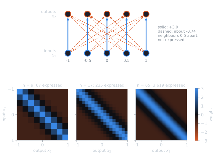
The same CPPN, queried without change on rows of 5, 9, 17, 33 and 65 neurons, gives:
| Neurons per row | Potential connections | Expressed | Excitatory | $w(0 \to 0)$ | $w(-0.5 \to 0)$ | Most active output |
|---|---|---|---|---|---|---|
| 5 | 25 | 17 | 5 | 3.0 | 0 | $-0.5$ (tie) |
| 9 | 81 | 67 | 25 | 3.0 | 0 | $-0.5$ |
| 17 | 289 | 235 | 79 | 3.0 | 0 | $-0.5$ |
| 33 | 1,089 | 933 | 333 | 3.0 | 0 | $-0.5$ |
| 65 | 4,225 | 3,619 | 1,363 | 3.0 | 0 | $-0.5$ |
Two things stay fixed as the substrate grows. The weight between two given positions is the same at every resolution, because it is a function of the positions and not of the indices; the grids here are nested, so positions such as 0 and $-0.5$ exist at every size. And the network's behaviour is the same. The last column is a one-dimensional version of the visual discrimination task described below: a large object covers $[-0.75, -0.25]$, a small one a third as wide is centred at 0.5, input activation is scaled by $8/(n - 1)$ so that a finer grid does not deliver more total input, and the most active output should mark the centre of the large object. It does at every resolution from 9 upward. At 5 neurons both objects cover a single input node, so they are indistinguishable and the two centres tie at activation 4.520 (the script reports the first). At 65 neurons the network has 3,619 expressed connections, and none of them was set individually.
Visual discrimination at nine million connections
Gauci and Stanley (2007) demonstrated HyperNEAT on the task at the top of this article. The substrate was two 11 by 11 sheets, a visual field of on-off sensors and a target field of outputs, and the network had to make the output at the centre of the larger of two squares (one three times the width of the other) the most active. Each CPPN was scored on 75 placements of the two objects. With a population of 100 for 300 generations, averaged over 20 runs, HyperNEAT found near-perfect and often perfect solutions. The comparison method, a NEAT variant that evolved the 14,641 weights directly, did not learn the task effectively.
The best CPPN of each generation was then queried at 33 by 33 and 55 by 55, with input activation scaled for the smaller cells, and evaluated without further evolution on all valid object placements, many of which do not exist at 11 by 11. Two sheets of $55 \times 55$ neurons have up to $55^4 = 9{,}150{,}625$ connections, and the networks scaled almost perfectly: performance at the higher resolutions was not significantly different from 11 by 11 after the second generation. High-quality CPPNs expressed 8.3 million connections on average at 55 by 55. The genomes were small. Taking solutions with average distance from the target under 0.25, the average CPPN had only 24 connections, while its 11 by 11 substrate had on average 12,827 of the 14,641 possible connections, a ratio of about 534 (Gauci and Stanley, 2007, §5). Stanley, D'Ambrosio and Gauci (2009) give the full account of the method, with the visual discrimination task and a food-gathering robot task.
ES-HyperNEAT: letting the CPPN place the neurons
In HyperNEAT the experimenter decides how many hidden neurons there are and where they sit, and a poor choice limits what the CPPN can express. Risi and Stanley (2012) proposed evolvable-substrate HyperNEAT (ES-HyperNEAT), which deduces the placement and density of hidden neurons from information already implicit in the CPPN's pattern of weights. In outline, it examines the weight pattern at increasing resolution with a quadtree, subdividing where the pattern varies and placing neurons there, so that regions where the pattern carries more information receive more neurons. The paper tests the method on multi-task, maze navigation and modular retina domains and reports networks with neural topography and geometric regularity.
The cost of a bias toward regularity
An indirect encoding is a bet that the problem is regular. Clune, Stanley, Pennock and Ofria (2011) measured what happens when the bet fails, on three problems whose regularity they could adjust: matching a target set of weights, mirroring input bits to outputs, and evolving gaits for a simulated four-legged robot, made less regular by giving it faulty joints. In all three, HyperNEAT's performance rose with the regularity of the problem, and it outperformed direct-encoding controls (fixed-topology NEAT, and on the robot also NEAT itself) on the most regular versions. When regularity was low, the direct encodings outperformed HyperNEAT.
The clearest case was a target-weights problem in which 90% of the weights shared one value and 10% had random values. Within a few generations HyperNEAT set all its weights to the common value, and in the remaining hundreds of generations it never made the exceptions needed for the other 10%. The authors' remedy, HybrID, runs HyperNEAT first and then refines the resulting weights with a direct encoding. It matched HyperNEAT on regular problems and outperformed it on problems with some irregularity, which suggests that an indirect encoding may work best as the first stage of a search, laying down the regular pattern, with a separate process, perhaps learning, adding the irregular details (Clune et al., 2011).
Two other limits follow from the design. The substrate's geometry is supplied by the experimenter, and HyperNEAT is only as good as the layout's match to the task; ES-HyperNEAT relaxes this for hidden neurons, not for inputs and outputs. And querying a CPPN for every potential connection costs time proportional to the number of connections: Gauci and Stanley (2007) report 3.2 minutes on a 2.0 GHz processor to build an eight-million-connection network, though only 0.09 seconds to run it on one trial.
Related ideas
A CPPN is an evolved function of coordinates, much as a genetic program is an evolved expression; the difference is that the CPPN is a graph of weighted sums and canonical functions and is grown by NEAT. Searching for variety rather than for one objective, as Picbreeder's users did, is the subject of MAP-Elites and novelty search. The course's soft-robot project encoded its 5 by 5 voxel bodies directly, voxel by voxel, alongside NEAT controllers, and evolutionary robotics covers the wider field of evolving bodies and controllers.
References
- Clune, J., Stanley, K. O., Pennock, R. T., and Ofria, C. (2011). On the performance of indirect encoding across the continuum of regularity. IEEE Transactions on Evolutionary Computation, 15(3), 346–367.
- Gauci, J., and Stanley, K. O. (2007). Generating large-scale neural networks through discovering geometric regularities. In Proceedings of the 9th Annual Conference on Genetic and Evolutionary Computation (GECCO 2007), 997–1004. ACM.
- Risi, S., and Stanley, K. O. (2012). An enhanced hypercube-based encoding for evolving the placement, density, and connectivity of neurons. Artificial Life, 18(4), 331–363.
- Secretan, J., Beato, N., D'Ambrosio, D. B., Rodriguez, A., Campbell, A., Folsom-Kovarik, J. T., and Stanley, K. O. (2011). Picbreeder: A case study in collaborative evolutionary exploration of design space. Evolutionary Computation, 19(3), 373–403.
- Stanley, K. O. (2007). Compositional pattern producing networks: A novel abstraction of development. Genetic Programming and Evolvable Machines, 8(2), 131–162.
- Stanley, K. O., D'Ambrosio, D. B., and Gauci, J. (2009). A hypercube-based encoding for evolving large-scale neural networks. Artificial Life, 15(2), 185–212.