Two strains of bacteria grow in a flask of nutrient broth with food to spare. One divides slightly faster than the other. Nothing struggles, nothing starves, and no individual is killed, yet after enough generations the faster strain makes up nearly the whole culture. Richard Lewontin used this example to make a point about Darwin's theory: competition for scarce resources is not part of its logic (Lewontin, 1970). What the theory needs is less dramatic and more general, and it is exactly the part that evolutionary algorithms borrow.
This article sets out the biology as biologists state it, then says for each idea what an evolutionary algorithm (EA) keeps, what it simplifies, and what it leaves out. Eiben and Smith (2015, ch. 2) give a short account of the same inspiration, explicitly simplified. The aim here is to be precise about the simplifications, because several common misunderstandings about EAs start with a biological word used in a sense biology does not give it. The limits of the evolutionary metaphor take up the consequences.
Selection in three conditions
Darwin (1859) argued that species change over time by natural selection acting on heritable variation. He did not know how inheritance worked. Lewontin (1970) reduced the argument to three principles that make no assumption about mechanism:
- Variation. Individuals in a population differ in their morphology, physiology, and behavior.
- Differential fitness. Different variants survive and reproduce at different rates.
- Heritability. Offspring resemble their parents, so that parents' fitness is correlated with their offspring's.
While all three hold, the population changes. Lewontin stressed how little the principles specify. Inheritance can be genetic, cytoplasmic, or cultural, and the reason one variant out-reproduces another is left open. Any set of entities with variation, reproduction, and heritability can evolve, which is why the principles transfer to programs and bitstrings at all.
What an EA keeps. All three, deliberately. A population of candidate solutions supplies variation, a selection operator makes reproduction depend on a score, and copying with small changes makes offspring resemble their parents.
What it adds. The principles say that the population changes. They do not say that it improves, still less that it finds anything best. An EA becomes an optimizer only because its designer fixes what counts as fitness and holds it constant, as the next section explains.
Fitness is reproductive success
In biology, fitness is a measure of reproductive success: roughly, the expected number of offspring an individual or a genotype contributes to the next generation, usually expressed relative to the rest of the population (Futuyma and Kirkpatrick, 2017). Three features of this definition matter for computing.
- Fitness is an outcome, not a cause. No organism is scored. Fitness describes how many descendants a variant leaves, which is the result of everything it does in its environment. "Survival of the fittest" is therefore close to circular if read as a law, and biologists do not use it as one.
- Fitness is relative and environment-dependent. A variant that is fitter in one environment can be less fit in another, and the environment includes the other members of the population. When the advantage of a variant depends on how common it is, fitness changes as the population changes.
- Fitness is a property of a variant in context, not of a design. Selection favors whatever leaves more descendants now. It does not look ahead.
What an EA does instead. An EA defines an explicit fitness function that maps each candidate to a number before reproduction happens, and uses that number to decide who reproduces (parent selection) and who stays in the population (survivor selection) (Eiben and Smith, 2015, ch. 5). The fitness function is fixed for the whole run in most EAs. It is a property of the candidate alone, so it does not depend on what else is in the population, and it encodes what the designer wants.
The two meanings meet in one place. Under fitness-proportional selection, a population of $N$ individuals with fitness values $f_1, \dots, f_N$ chooses each parent with probability $f_i / \sum_j f_j$. Over $N$ draws, individual $i$ receives on average
$$N \cdot \frac{f_i}{\sum_j f_j} = \frac{f_i}{\bar{f}}$$
copies, where $\bar{f}$ is the population's mean fitness. That ratio is exactly the biologist's relative fitness: expected offspring compared with the average. Other schemes, such as tournament selection, give each individual an expected number of offspring that depends only on its rank, and the number the fitness function returns is then just an ordering. Either way, the algorithm's "fitness" is an engineering quantity that becomes reproductive success only through the selection operator. Selection pressure is the measure of how strongly that operator favors the best.
What an EA discards. Coevolution aside, the moving environment: in nature the target shifts as other species evolve. Competitive coevolution restores this feature on purpose, and with it some of the instability that natural evolution shows, such as Red Queen dynamics.
Selection as arithmetic
Relative fitness becomes a prediction once it is written as a recursion. Take the simplest case population genetics studies: a large population of haploid individuals (one copy of each gene) of two types, A and a, with relative fitness $w_A = 1 + s$ and $w_a = 1$. The number $s$ is the selective advantage of A: $s = 0.1$ means that A leaves 10% more offspring on average. Let $p$ be the frequency of A in one generation.
- Each type contributes offspring in proportion to its frequency times its fitness: $p\, w_A$ for A and $(1 - p)\, w_a$ for a.
- The total, which is the population's mean fitness, is $\bar w = p\, w_A + (1 - p)\, w_a = 1 + s p$.
- Dividing A's share by the total gives its frequency in the next generation:
$$p' = \frac{p\, w_A}{\bar w} = \frac{p (1 + s)}{1 + s p}.$$
This is the same expression as fitness-proportional selection, $f_i / \bar f$ copies per individual, written for two types instead of $N$ individuals.
The recursion has a closed form. Divide the equation for $p'$ by the same equation for $1 - p' = (1 - p)/(1 + sp)$: the denominators cancel and the odds $p/(1 - p)$ are multiplied by exactly $1 + s$ each generation. After $t$ generations,
$$\frac{p_t}{1 - p_t} = (1 + s)^t\, \frac{p_0}{1 - p_0}.$$
Starting from $p_0 = 0.01$ with $s = 0.1$, the odds start at $1/99$ and must reach $99$ for A to make up 99% of the population, a factor of $99^2 = 9{,}801$. That takes $\ln 9{,}801 / \ln 1.1 \approx 96.4$ generations, so the frequency first exceeds 0.99 in generation 97. The script tools/experiments/evolution/selection_dynamics.py iterates the recursion and agrees with the closed form at every step (values rounded to four decimals):
| Generation $t$ | $p_t$ | $\bar w_t$ |
|---|---|---|
| 0 | 0.0100 | 1.0010 |
| 10 | 0.0255 | 1.0026 |
| 20 | 0.0636 | 1.0064 |
| 30 | 0.1498 | 1.0150 |
| 40 | 0.3137 | 1.0314 |
| 50 | 0.5425 | 1.0542 |
| 60 | 0.7546 | 1.0755 |
| 80 | 0.9539 | 1.0954 |
| 100 | 0.9929 | 1.0993 |
The curve is an S shape. For 30 generations A is rare and its frequency grows by about 10% per generation in relative terms, barely visible in absolute terms. Most of the change happens in the middle, and the last stretch is slow again, because a has become rare and is replaced at a rate proportional to its own small frequency.
Mean fitness rises throughout, and the reason can be stated in one line. With constant fitness values, $\bar w' = \sum_i p'_i w_i = \sum_i p_i w_i^2 / \bar w$, so
$$\bar w' - \bar w = \frac{\sum_i p_i w_i^2 - \bar w^2}{\bar w} = \frac{\operatorname{Var}(w)}{\bar w} \ge 0.$$
Selection on fixed fitness values raises mean fitness by the variance in fitness divided by its mean, and stops raising it only when the variance is gone. In the first generation of the table, $\operatorname{Var}(w) = s^2 p (1 - p) = 0.000099$, and $\bar w$ rises from 1.0010 to 1.0011. The condition "fixed fitness values" is exactly the one an EA meets and nature does not; the limits of the evolutionary metaphor gives a case where selection lowers mean fitness instead.
The same arithmetic inside an EA. Suppose a population of 50 OneMax strings all have fitness 50, except one copy of a string with an extra 1, fitness 51. Under fitness-proportional selection its advantage is $s = 1/50 = 0.02$, and the recursion says it needs $\ln(49^2)/\ln 1.02 \approx 393$ generations, 394 when iterated, to go from 1 copy in 50 to 49 in 50. Under binary tournament selection, the better type wins any tournament it enters, and it is absent from a tournament only when both entrants are the other type, so $p' = 1 - (1 - p)^2 = p(2 - p)$. At small $p$ this doubles the frequency every generation, whatever the fitness values are, and the same takeover needs 8 generations: 0.020, 0.040, 0.078, 0.149, 0.276, 0.476, 0.726, 0.925, 0.994.
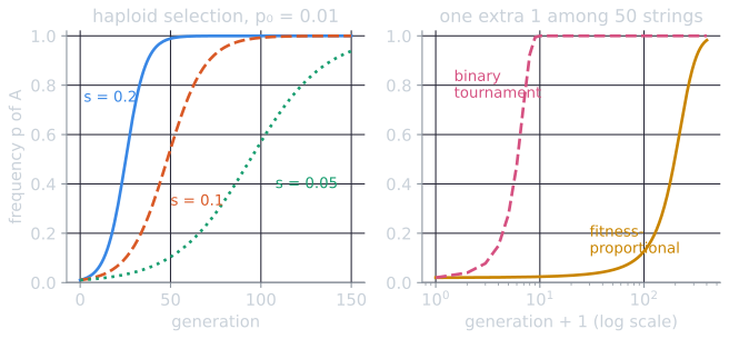
The contrast is the deterministic version of the drift experiment later in this article, in which fitness-proportional selection on OneMax lost dozens of loci that tournament selection kept.
Heredity: genes, alleles, genotype, phenotype
Darwin's mechanism needed heredity but lacked a theory of it. Gregor Mendel's crosses of garden peas, published in 1866, showed that traits are passed on as discrete units that do not blend (Mendel, 1866). The units came to be called genes.
- A gene is a unit of heredity, in molecular terms a stretch of DNA that is transcribed into a functional product.
- A locus is the position of a gene on a chromosome.
- An allele is one of the alternative variants that can occupy a locus. Most animals are diploid, carrying two copies of each chromosome and so two alleles at each locus, one from each parent.
Wilhelm Johannsen introduced the terms in 1909 and set out in English the distinction between genotype, the hereditary constitution of an organism, and phenotype, its observable characteristics (Johannsen, 1911). The phenotype is produced by development, the long process by which a genotype builds an organism in interaction with its environment. Selection acts on phenotypes. Only genotypes are inherited.
What an EA keeps. The vocabulary, mapped onto data structures (Eiben and Smith, 2015, ch. 3). In a genetic algorithm on bitstrings, the string is the chromosome or genotype, each position is a locus, and the value 0 or 1 at a position is its allele. The phenotype is the solution the string represents, such as a set of real-valued parameters decoded from the bits by a binary or Gray code. Fitness is computed from the phenotype.
What it simplifies. The genotype-to-phenotype map is usually a direct decoding with no development, no environmental influence, and no noise. EAs are almost always haploid: one string per individual, no dominance, no pairs of alleles. A few representations reintroduce indirect, development-like mappings, such as the grammar-based mappings of grammatical evolution, which turn an integer string into a program, and the compositional pattern-producing networks of HyperNEAT, where a small genotype generates a large, regular phenotype.
What it can break. Biological inheritance does not pass on traits an organism acquires in its lifetime; the phenotype does not write back to the genotype. An EA is free to break this rule. A memetic algorithm improves each offspring with a local search such as hill climbing and may write the improved solution back into the genotype, which is Lamarckian inheritance. Alternatively, it may keep the original genotype but score it by the improved phenotype, which is called the Baldwinian variant (Eiben and Smith, 2015, ch. 10).
Variation: mutation and recombination
Mutation in biology is any change in the DNA sequence: a substituted nucleotide, an insertion or deletion, a duplicated gene, a rearranged chromosome. Mutation is random with respect to its effect: it does not occur preferentially where it would help. Most mutations that affect fitness are harmful, and many have little or no effect. Rates are low. In humans, Kong and colleagues (2012) measured an average of $1.20 \times 10^{-8}$ new mutations per nucleotide per generation, which over a diploid genome of about $6 \times 10^9$ nucleotides is roughly 70 new mutations per child.
Recombination shuffles existing variation. In sexual reproduction, meiosis assigns each gamete one copy of each chromosome, chosen independently, and crossing over exchanges segments between the two copies of a chromosome before they separate. Each offspring therefore carries a new combination of its parents' alleles. Because the paired chromosomes are aligned gene by gene, crossing over normally exchanges corresponding segments.
What an EA keeps. Both kinds of variation, as operators the designer chooses (see crossover and mutation operators). Bit-flip mutation flips each bit independently with a small probability, and one-point or uniform crossover combines two parent strings position by position, much as aligned chromosomes do.
What it changes. The rates and the targets. A common default flips each bit with probability $1/L$ for a string of length $L$, so each offspring carries one mutation on average. For $L = 100$, the per-site rate is 0.01, nearly a million times the human rate of $1.2 \times 10^{-8}$. Mutation in an EA need not be blind to the problem: operators are designed for a representation, and self-adaptive evolution strategies evolve their own mutation step sizes. Recombination need not respect any biological constraint. It can combine three parents, average real-valued vectors, or be omitted entirely.
Heritability: how much of selection is passed on
Lewontin's third condition, heritability, is not all or nothing. Offspring resemble their parents more or less closely, and the degree sets how much of a selected difference reaches the next generation. Plant and animal breeders measure it with two numbers. The selection differential $S$ is how much better the selected parents are than the population they came from, measured on the trait being selected. The response $R$ is how much better their offspring are than that same population. The ratio $R/S$ is the realized heritability.
An EA with a noisy fitness function shows why the ratio can be well below 1. Suppose each candidate has a true quality $g$, but every evaluation returns $z = g + e$, where the noise $e$ is drawn independently each time with mean 0 and variance $\sigma_e^2$. Selection sees only $z$. The derivation takes three steps.
- What selection on $z$ does to $g$. The best linear prediction of $g$ from $z$ is $\bar g + h^2 (z - \bar z)$, where the slope is $h^2 = \operatorname{cov}(g, z) / \operatorname{Var}(z) = \sigma_g^2 / (\sigma_g^2 + \sigma_e^2)$, the share of the measured variance that is real. The prediction is exact when $g$ and $e$ are normally distributed and close to exact for sums of many bits. Averaging it over the selected parents, whose mean $z$ exceeds $\bar z$ by $S$, gives a mean true quality of $\bar g + h^2 S$.
- What crossover passes on. On a problem where every bit contributes separately to $g$, such as OneMax, uniform crossover takes each bit from one parent or the other with probability $\tfrac12$, so a child's expected $g$ is the mean of its two parents' $g$. Averaged over all children, the population of offspring has mean true quality $\bar g + h^2 S$.
- What the next evaluation sees. The noise has mean 0, so the offspring's mean measured fitness is also $\bar g + h^2 S$, and the response is
$$R = h^2 S.$$
This is known in breeding as the breeder's equation. Here $h^2$ plays the role of heritability, and in this setting it is fixed by the noise: half of the variance is noise when $\sigma_e^2 = \sigma_g^2$, and then only half of the selection differential is passed on.
The script tools/experiments/evolution/selection_dynamics.py checks the equation on OneMax with 100 bits and a population of 1,000. In a random population $g$ has variance $100 \cdot \tfrac14 = 25$. Truncation selection keeps the better half by measured fitness, uniform crossover of random pairs of the selected parents makes 1,000 children without mutation, and the children are measured with fresh noise. Thirty seeded runs per noise level, median with interquartile range in brackets, rounded to two or three decimals:
| Noise $\sigma_e$ | $h^2 = 25/(25 + \sigma_e^2)$ | $S$ | $R$ | $R/S$ |
|---|---|---|---|---|
| 0 | 1 | 4.00 | 3.99 | 1.00 [0.97, 1.02] |
| 5 | 0.5 | 5.67 | 2.83 | 0.51 [0.46, 0.53] |
| 10 | 0.2 | 8.93 | 1.60 | 0.18 [0.15, 0.25] |
The selection differential grows with the noise, because the measured values spread out (truncation to the better half of a normal distribution gives $S \approx 0.80\, \sigma_z$), yet the response shrinks. Much of what selection picks out is luck in the measurement, and luck is not inherited. This is the precise sense in which noisy evaluation weakens an EA: it lowers the heritability of fitness. Selecting harder raises $S$, but only the fraction $h^2$ of the extra differential is passed on; raising $h^2$ improves every generation's return, for example by averaging $k$ repeated evaluations of each candidate, which divides $\sigma_e^2$ by $k$.
Genetic drift
Selection is not the only force that changes allele frequencies. In a finite population, which individuals happen to reproduce is partly a matter of chance, so the frequency of an allele wanders from generation to generation even when it has no effect on fitness. This is genetic drift. Drift eventually fixes or eliminates every neutral allele. A neutral allele at frequency $p$ becomes fixed, present in every individual, with probability $p$. Drift is stronger in small populations. A common rule of thumb is that selection dominates an allele's fate only when its selective advantage $s$ is large compared with the reciprocal of the population size; when $s$ is comparable to $1/N$ or smaller, the allele behaves almost as if it were neutral (Futuyma and Kirkpatrick, 2017). Kimura (1968) argued that much of evolutionary change at the molecular level is the fixation of neutral mutations by drift, not adaptation.
Drift against selection, in numbers
The rule of thumb can be made exact enough to compute with. The Wright-Fisher model adds sampling to the recursion of the previous section. A population has exactly $N$ haploid individuals. To form the next generation, each of $N$ slots is filled independently by a copy of type A with probability $p(1+s)/(1+sp)$, the frequency that selection alone would give, so the number of A in the next generation is a binomial draw. Selection sets the expected direction and the binomial draw adds noise whose size depends on $N$.
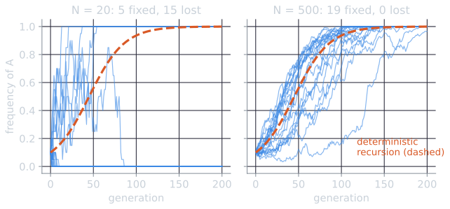
Whether A eventually takes over can be computed with the diffusion approximation, which treats $p$ as a continuous quantity that moves a little each generation. Two numbers describe one generation's move.
- The mean change is $p(1+s)/(1+sp) - p = sp(1-p)/(1+sp) \approx s p (1 - p)$ for small $s$.
- The variance of the change is that of a binomial frequency, $q(1-q)/N \approx p(1-p)/N$, where $q$ is the probability used for the draw.
Let $u(p)$ be the probability that A is eventually fixed when its frequency is $p$. One generation later the frequency is $p + \Delta p$, and the eventual outcome is the same random event, so $u(p)$ equals the average of $u(p + \Delta p)$. Expanding $u(p + \Delta p)$ to second order and averaging,
$$u(p) \approx u(p) + u'(p)\, \mathrm{E}[\Delta p] + \tfrac12 u''(p)\, \mathrm{E}[\Delta p^2],$$
and with the two numbers above, after cancelling $u(p)$ and dividing by $p(1-p)$:
$$s\, u'(p) + \frac{1}{2N} u''(p) = 0.$$
This says $u'' = -2Ns\, u'$, so $u'(p) = c\, e^{-2Nsp}$ for a constant $c$. Integrating and imposing $u(0) = 0$ (A already lost) and $u(1) = 1$ (A already fixed) gives
$$u(p) = \frac{1 - e^{-2Nsp}}{1 - e^{-2Ns}}.$$
Everything in the formula depends on $s$ and $N$ only through their product $Ns$, which is the exact form of the rule of thumb. Three cases show it.
- Neutral, $s \to 0$. Both exponentials expand to first order and $u(p) \to p$: a neutral allele fixes with probability equal to its frequency, as stated above.
- Strong selection, $Ns \gg 1$. The denominator is close to 1. A single new copy, $p = 1/N$, fixes with probability $1 - e^{-2s} \approx 2s$. A new mutation with a 5% advantage is lost about nine times in ten, however large the population, because it starts as one copy and can be lost by chance before selection has had time to act.
- Harmful, $s < 0$ with $N|s| \gg 1$. The probability falls off exponentially in $N|s|$. Small populations can fix harmful alleles; large ones almost never do.
The script tools/experiments/evolution/selection_dynamics.py checks the formula by simulation: for each $N$ and $s$, 30 seeded batches of 2,000 populations, each started with one copy of A.
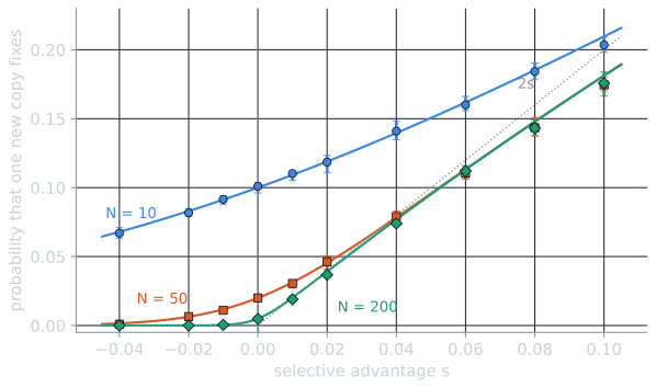
The simulated and approximate values agree to within 0.007 everywhere in this range: for $N = 50$ and $s = 0.02$ the simulation gives 0.046 and the formula 0.045; for $N = 200$ and $s = 0.1$ they are 0.176 and 0.181, the formula's small excess coming from the diffusion approximation itself, which keeps only the mean and variance of each generation's change and is most accurate when $s$ is small. For $N = 20$, $s = 0.05$ and $p_0 = 0.1$, the case on the left of the trajectory figure, the formula gives 0.210, so about 4 of the 20 populations should fix A; 5 did. For $N = 500$ it gives 0.993.
EA populations are tiny by biological standards, typically tens to hundreds of individuals, so drift is strong. The script tools/experiments/evolution/neutral_drift.py in the site repository measures it. Each run uses $N = 50$ random bitstrings of length 20 and no mutation, so the only sources of change are selection and sampling. All results are over 30 seeded runs.
Neutral, no crossover. Every individual has the same fitness, so each generation draws 50 parents uniformly at random with replacement. This is the haploid Wright-Fisher model of population genetics. Every run ended with all 50 individuals descended from a single founder, after a median of 95.5 generations (interquartile range 71 to 128.5; minimum 42, maximum 228). Coalescent theory predicts a mean of $2N(1 - 1/N) = 98$ generations; the 30 runs averaged 107.3, within the large run-to-run spread.
Neutral, uniform crossover. With each bit of a child taken from one of two random parents, the 20 loci drift almost independently. The population still became uniform in every run, after a median of 199.5 generations (interquartile range 183 to 219).
Weak selection on OneMax. With strings of length 100 and fitness equal to the number of ones (the OneMax problem), every 1 is the right allele. Under fitness-proportional selection with uniform crossover, every run converged to a single string, after a median of 253 generations, and a median of 30 of the 100 loci were fixed at the wrong allele (interquartile range 28 to 33). No run found the optimum. Under binary tournament selection the population converged in a median of 35 generations with a median of 2 wrong loci (interquartile range 1 to 2), and 5 of 30 runs found the optimum.
The rule of thumb explains the difference. Under fitness-proportional selection, carrying a 1 at one locus adds 1 to a fitness of about 50 to 70, a relative advantage of about $1/50$ to $1/70$, which is no larger than $1/N = 0.02$. Each locus is close to neutral, and drift fixes many of them at 0 before selection can act. Tournament selection uses only comparisons, so a one-bit difference decides any contest between two individuals that are otherwise tied, however large their fitness values are. Part of what EA practitioners call premature convergence is drift, not too much selection: the population loses alleles by chance, and without mutation nothing can bring them back. Mutation, larger populations, and diversity-preserving schemes such as island models and speciation are the usual remedies.
The modern synthesis
Mendelian genetics and Darwinian selection at first looked like rivals. Early Mendelians saw discrete mutations, not gradual selection, as the driver of change. Between about 1918 and 1932, Ronald Fisher, Sewall Wright, and J. B. S. Haldane showed mathematically that Mendelian inheritance and selection on small differences are compatible, founding population genetics (Fisher, 1930; Wright, 1931). In the following decade, naturalists and paleontologists brought evidence from their fields into the same framework. Julian Huxley's book named the result the modern synthesis (Huxley, 1942). Its core claims are that evolution is change in allele frequencies within populations; that the change is driven by mutation, recombination, selection, drift, and migration; and that the large differences between species accumulate from these small changes over long periods.
Classical EAs sit squarely inside this picture. A genetic algorithm is a population-genetics model with a chosen fitness function: a fixed population of haploid genotypes, allele frequencies changed by selection and drift, and new variation supplied by mutation and recombination. Wright's image of populations moving across a surface of fitness values became the fitness landscape that EA researchers use to reason about difficulty. Later developments in biology, such as the neutral theory, the role of development in shaping which variants can arise, and the genomics of gene regulation, have had less influence on mainstream EAs, though each has inspired research directions.
Summary: what an EA keeps, simplifies, and discards
| Biology | In a typical EA | Status |
|---|---|---|
| Variation, differential fitness, heritability | Population, selection operator, copying with variation | Kept |
| Fitness as realized reproductive success, relative and environment-dependent | Explicit fitness function, fixed for the run, scored per candidate | Replaced |
| Variable population size, overlapping generations | Fixed size; generational or steady-state replacement | Simplified |
| Diploid genotypes, dominance | One haploid string per individual | Simplified |
| Development from genotype to phenotype | Direct decoding; indirect encodings are the exception | Mostly discarded |
| Mutation random with respect to effect, about $10^{-8}$ per site | Designed operators, typically one change per offspring, sometimes self-adapted | Changed |
| Recombination of aligned chromosomes in meiosis | Crossover of any kind, any number of parents, or none | Generalized |
| Acquired traits not inherited | Lamarckian writing-back allowed in memetic algorithms | Optional |
| Genetic drift | Present and strong, since populations are small | Kept, usually unintentionally |
| Changing environment, coevolving species | Fixed objective, except in coevolutionary algorithms | Discarded by default |
Eiben and Smith (2015, §2.1) summarize the borrowed analogy as a correspondence between natural evolution and problem solving: environment to problem, individual to candidate solution, fitness to quality. The table shows how much each side of that correspondence has been reshaped. What remains is the logic Lewontin identified, applied to a population that the designer sizes, scores, and controls.
References
- Darwin, C. (1859). On the Origin of Species by Means of Natural Selection, or the Preservation of Favoured Races in the Struggle for Life. John Murray.
- Eiben, A. E., and Smith, J. E. (2015). Introduction to Evolutionary Computing, 2nd ed., chapters 2, 3, 5, and 10. Springer.
- Fisher, R. A. (1930). The Genetical Theory of Natural Selection. Clarendon Press.
- Futuyma, D. J., and Kirkpatrick, M. (2017). Evolution, 4th ed. Sinauer Associates.
- Huxley, J. (1942). Evolution: The Modern Synthesis. George Allen and Unwin.
- Johannsen, W. (1911). The genotype conception of heredity. The American Naturalist, 45(531), 129–159.
- Kimura, M. (1968). Evolutionary rate at the molecular level. Nature, 217(5129), 624–626.
- Kong, A., Frigge, M. L., Masson, G., Besenbacher, S., Sulem, P., Magnusson, G., et al. (2012). Rate of de novo mutations and the importance of father's age to disease risk. Nature, 488(7412), 471–475.
- Lewontin, R. C. (1970). The units of selection. Annual Review of Ecology and Systematics, 1, 1–18.
- Mendel, G. (1866). Versuche über Pflanzen-Hybriden. Verhandlungen des naturforschenden Vereines in Brünn, 4, 3–47.
- Wright, S. (1931). Evolution in Mendelian populations. Genetics, 16(2), 97–159.