A genetic algorithm in its classic form works on bit strings, but many problems are stated in real numbers: a temperature between 20.1 and 45.6 degrees, a coordinate between $-5.12$ and $5.12$. Before the algorithm can search such a space, each real variable has to be mapped to a block of bits, and the mapping decides which candidates are reachable, how finely the space is sampled, and which candidates a single mutation can reach from a given one. This article covers the standard binary mapping and its precision, the problem of Hamming cliffs that it creates, the Gray code that removes them, and what experiments show about the difference. It assumes the simple genetic algorithm.
Mapping an interval to bit strings
Let a variable $x$ lie in an interval $[L, U]$, and give it $n$ bits. An $n$-bit string $b_1 b_2 \dots b_n$, read with the most significant bit first, is an integer
$$k = \sum_{i=1}^{n} b_i \, 2^{\,n-i}, \qquad 0 \le k \le 2^n - 1.$$
The standard linear decoding sends $k = 0$ (all zeros) to $L$ and $k = 2^n - 1$ (all ones) to $U$, with equally spaced points between:
$$x = L + k \, \varepsilon, \qquad \varepsilon = \frac{U - L}{2^n - 1}.$$
The step $\varepsilon$ is the precision of the encoding: the distance between neighboring representable values. A real value that falls between grid points is represented by the nearest one, so the representation error is at most $\varepsilon / 2$.
Three worked examples, each computed and checked:
- Precision from length. For $1 \le x \le 16$ with $n = 6$ bits, $\varepsilon = 15 / 63 = 0.238$ to three places. Truncating this to 0.23 understates the step.
- Precision for an 8-bit variable. For $20.1 \le x \le 45.6$ with $n = 8$, $\varepsilon = 25.5 / 255 = 0.1$ exactly, so the 256 representable values are 20.1, 20.2, and so on up to 45.6.
- Decoding and encoding. For $2 \le x \le 17$ with $n = 4$, $\varepsilon = 15 / 15 = 1$. The string 1010 is $k = 8 + 2 = 10$, which decodes to $x = 2 + 10 \times 1 = 12$. Going the other way, $x = 12$ gives $k = (12 - 2) / 1 = 10$, whose binary form is 1010. (A common slip writes 1100, which is 12, the value of $x$ rather than of $k$.)
Choosing the length. To guarantee a precision of at most $\varepsilon$, the number of bits must satisfy $(U - L)/(2^n - 1) \le \varepsilon$, so
$$n = \left\lceil \log_2\!\left(\frac{U - L}{\varepsilon} + 1\right) \right\rceil.$$
On $[-5.12, 5.12]$, a precision of 0.01 needs $\lceil \log_2 1025 \rceil = 11$ bits, because 10 bits give $10.24 / 1023 = 0.01001$, just over the target. A precision of 0.001 needs 14 bits. Some authors divide by $2^n$ instead of $2^n - 1$, so that 10 bits on $[-5.12, 5.12]$ give a step of exactly 0.01 and the upper bound itself is not representable. De Jong (1975) discretized his test functions with a power of two of points on each axis, for example 1,024 points on $[-5.12, 5.12]$ at a nominal resolution of 0.01, as described in a binary GA on De Jong's test functions. The two conventions differ only in whether $U$ is on the grid.
When a variable takes a fixed set of values whose count is not a power of two, some bit patterns are left over. Whitley (1994) gives the example of a variable with exactly 1,200 values: it needs 11 bits, and $2^{11} - 1200 = 848$ of the patterns represent nothing. They must be given no evaluation or a worst-possible one, or mapped to legal values so that some values are represented twice; Whitley treats the choice as part of designing the evaluation function.
Several variables
A candidate with several variables is encoded by concatenating their blocks. The course's second assignment, examined in a binary GA on De Jong's test functions, encoded De Jong's three-variable sphere function F1 with 8 bits per variable, a 24-bit string. On $[-5.12, 5.12]$ with 8 bits, $\varepsilon = 10.24 / 255 = 0.040157$. The string
10000010 10000011 01111101
splits into $k = 130, 131, 125$, which decode to $x \approx (0.1004, 0.1405, -0.1004)$, with $\sum x_i^2 = 0.0399$. That was the best 8-bit solution the submitted report gave for F1.
Concatenation has a consequence for crossover. One-point crossover cuts the string at a single position, so blocks that sit next to each other on the string are more likely to be inherited together than blocks at opposite ends. Whether that matters depends on whether the variables interact, a question taken up by the schema theorem.
Hamming cliffs
Bit-flip mutation at the usual low rates changes one bit or none in most offspring, so the candidates a mutation reaches most easily are those at Hamming distance 1, differing in a single bit. Under standard binary coding, Hamming distance and numerical distance can disagree badly. Adjacent integers can differ in every bit:
| $k$ | Binary | $x$ on the 8-bit grid of $[-5.12, 5.12]$ |
|---|---|---|
| 127 | 01111111 | $-0.020078$ |
| 128 | 10000000 | $+0.020078$ |
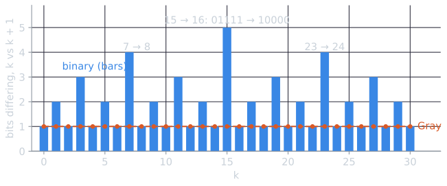
The two grid points closest to zero, where the sphere function has its minimum, are as far apart as two 8-bit strings can be. Moving from one to the other by mutation requires flipping all eight bits at once. Caruana and Schaffer (1988) called such a gap a Hamming cliff. Cliffs are not rare. Over all 255 pairs of adjacent integers on an 8-bit grid, 128 pairs differ in one bit, 64 in two, 32 in three, and so on, down to the single pair 127 and 128 that differs in all eight. The converse also holds: a single bit flip can move a long way. Flipping the leading bit of any string moves $k$ by 128, half the range.
The pattern is easier to see on 5 bits. Adding 1 to $k$ flips the trailing run of ones to zeros and the 0 before it to a 1, so the number of bits that change is one more than the number of trailing ones in $k$. Half of all integers end in 0 and change one bit, a quarter end in 01 and change two, and so on, up to $k = 15$ (01111), whose successor 16 (10000) differs in all five.
The reflected Gray code
A Gray code orders the bit strings so that consecutive integers always differ in exactly one bit. The usual one, the binary reflected Gray code, takes its name from its construction: the $n$-bit list is the $(n-1)$-bit list with a 0 prefixed, followed by the same list in reverse order with a 1 prefixed. Frank Gray patented it for pulse code communication (Gray, 1953). For three bits:
| $k$ | 0 | 1 | 2 | 3 | 4 | 5 | 6 | 7 |
|---|---|---|---|---|---|---|---|---|
| Binary | 000 | 001 | 010 | 011 | 100 | 101 | 110 | 111 |
| Gray | 000 | 001 | 011 | 010 | 110 | 111 | 101 | 100 |
The construction can be carried out by hand. Start from the 1-bit list 0, 1. Prefix it with 0, then append the list in reverse order prefixed with 1:
| Step | List |
|---|---|
| 1 bit | 0, 1 |
| 2 bits: 0 + (0, 1), then 1 + (1, 0) | 00, 01, 11, 10 |
| 3 bits: 0 + (00, 01, 11, 10), then 1 + (10, 11, 01, 00) | 000, 001, 011, 010, 110, 111, 101, 100 |
Each half of the list is a Gray code by the previous step, so consecutive entries within a half differ in one bit. At the join, the last entry of the first half and the first entry of the second half are the same $(n-1)$-bit string, with prefixes 0 and 1, so they too differ in one bit. Induction on $n$ gives the property for every length. The last entry, 100, also differs from the first, 000, in one bit, so the code is cyclic.
Conversion. From binary $b_1 \dots b_n$ to Gray $g_1 \dots g_n$, keep the first bit and XOR each later bit with the one before it:
$$g_1 = b_1, \qquad g_i = b_{i-1} \oplus b_i \quad (i = 2, \dots, n).$$
As an operation on integers, $g = k \oplus \lfloor k / 2 \rfloor$, that is, k ^ (k >> 1). The inverse accumulates XORs from the left:
$$b_1 = g_1, \qquad b_i = b_{i-1} \oplus g_i, \quad \text{so} \quad b_i = g_1 \oplus g_2 \oplus \dots \oplus g_i.$$
For example, $k = 10$ is 1010 in binary, and its Gray code is $1,\ 1 \oplus 0,\ 0 \oplus 1,\ 1 \oplus 0 = 1111$. Decoding 1111 gives $b = 1,\ 1 \oplus 1,\ 0 \oplus 1,\ 1 \oplus 1 = 1010$, back to 10. A 5-bit example, $k = 13$ (binary 01101), traced one position at a time in both directions:
| $i$ | $b_i$ | Encode: $g_i = b_{i-1} \oplus b_i$ | Decode: $b_i = g_1 \oplus \dots \oplus g_i$ |
|---|---|---|---|
| 1 | 0 | $g_1 = b_1 = 0$ | $0$ |
| 2 | 1 | $0 \oplus 1 = 1$ | $0 \oplus 1 = 1$ |
| 3 | 1 | $1 \oplus 1 = 0$ | $1 \oplus 0 = 1$ |
| 4 | 0 | $1 \oplus 0 = 1$ | $1 \oplus 1 = 0$ |
| 5 | 1 | $0 \oplus 1 = 1$ | $0 \oplus 1 = 1$ |
So 13 has the Gray code 01011, and decoding accumulates a running XOR of the Gray bits (each row's decode value is the previous row's value XOR $g_i$), recovering 01101. The rule has a simple reading: after the first bit, which is copied, a Gray bit is 1 exactly where the binary string changes value from the position before. In a GA, Gray coding changes only the step from bits to the integer $k$. The strings, the operators and the linear map from $k$ to $x$ stay the same.
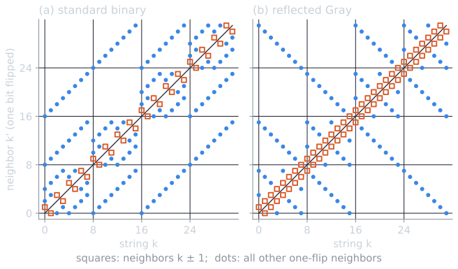
The cliff at the origin disappears: 127 and 128 have the Gray codes 01000000 and 11000000, one bit apart. What Gray coding does not do is make every one-bit move a small one. The eight integers one flip away from 127 are 126 and 128, its two grid neighbors, but also 0, 64, 96, 112, 120 and 124. Under binary they are 63, 95, 111, 119, 123, 125, 126 and 255. Both codes give each string $n$ neighbors spread over the whole range. Gray coding guarantees only that the two grid neighbors are among them.
A cliff that traps a local search
A small example shows what a cliff does to a search that moves by single bit flips. Minimize $f(k) = (k - 15)^2$ over the 5-bit integers $0, \dots, 31$. On the grid the function has one minimum, $k = 15$, and falls steadily toward it from both sides. Under standard binary, 15 is 01111 and its successor 16 is 10000. The five one-flip neighbors of 16 are 0, 17, 18, 20 and 24, with $f$ values 225, 4, 9, 25 and 81, all worse than $f(16) = 1$. So 16 is a local minimum under binary coding: no single bit flip improves it, although it sits next to the global minimum on the grid. Under Gray coding, 16 is 11000 and 15 is 01000, one flip apart, and 16 is not a local minimum.
Steepest descent makes the difference concrete. Starting from a string, move to the best of its five one-flip neighbors as long as that neighbor is strictly better, and stop otherwise. Run from each of the 32 starting strings:
| Coding | Strict local minima | Starts ending at 15 | Starts ending at 16 |
|---|---|---|---|
| Standard binary | 15, 16 | 17 | 15 |
| Reflected Gray | 15 | 32 | 0 |
Under binary, nearly half of the starts, including every start from 16 to 27, end on the wrong side of the cliff. From 24 (11000), for instance, the best flip clears the second bit and lands on 16 (10000), where the search stops. Under Gray coding every start reaches 15; from 24 (Gray 10100) the path is 24, 23, 16, 15, each step a single flip. A genetic algorithm is not a steepest-descent search, but at low mutation rates its offspring are mostly one or two flips from their parents, and the same trap applies to it whenever crossover cannot supply the missing bits.
The example is one case of a general rule. Gray coding's guarantee that both grid neighbors are one flip away has a precise consequence. Every point that is a local minimum under one-bit-flip moves in the Gray-coded space is also a local minimum on the grid itself (with neighbors $k \pm 1$ in each variable), because its grid neighbors are among its Gray neighbors. Gray coding can add no local minima beyond those of the grid; it can only remove some. Standard binary offers no such guarantee. On Rosenbrock's function F2 with 8 bits per variable, a grid of 65,536 points, the counts of strict local minima are:
| Neighborhood | Local minima |
|---|---|
| Grid neighbors, $k \pm 1$ in each variable | 103 |
| One bit flip, standard binary | 226 |
| One bit flip, Gray | 61 |
Binary coding more than doubles the number of local minima of the grid; Gray coding removes about 40 percent of them.
What the literature found
Caruana and Schaffer (1988) compared Gray and binary coding in genetic algorithms on function optimization problems and reported that Gray coding was generally better. They attributed the difference to Hamming cliffs, which make some moves between neighboring values hard under binary coding, and presented the cliff as one example of a hidden bias arising from the interaction between a representation and the operators that search it.
Theory placed limits on the claim. Over all possible functions, Gray and binary encodings must perform the same on average, by the No Free Lunch theorems, since each is just a relabeling of the same set of strings. Whitley (1999) made the trade-off precise. He defined a special class of functions that have the maximum possible number of local optima, proved that the reflected Gray code induces more optima than binary over that class, and concluded, from the No Free Lunch principle, that it induces fewer optima over all the remaining functions. Whitley's argument is that functions of limited complexity, with fewer than the maximum possible number of optima, are the ones worth optimizing, and over them Gray coding has the advantage on average. The result counts local optima under one-bit moves; it speaks most directly to search by mutation and local moves, and it does not promise that Gray coding wins on any particular function.
An experiment on De Jong's F1 and F2
The course's second assignment ran a binary GA on De Jong's functions, each configuration once. The script tools/experiments/evolution/gray_coding.py in the site repository repeats its GA with standard binary and Gray coding, 8 and 16 bits per variable, on F1 (the sphere, three variables on $[-5.12, 5.12]$) and F2 (Rosenbrock's function, two variables on $[-2.048, 2.048]$), with seeds 0 to 29. The GA is the assignment's: population 20, roulette-wheel selection on $1/(1 + f)$, two-point crossover with probability 0.9, bit-flip mutation at $1/L$, generational replacement without elitism, and the best value ever evaluated reported. Only the step from bits to integers differs between the two codings, so the binary runs at the assignment's budget repeat the 30-seed runs in a binary GA on De Jong's test functions exactly. The tables give the median best value found, with the interquartile range, and $A$, the probability that a randomly chosen Gray run ends lower than a randomly chosen binary run (Vargha and Delaney, 2000); 0.5 means no difference.
The GA, 50 generations (1,000 evaluations):
| Function | Bits | Binary | Gray | $A$ |
|---|---|---|---|---|
| F1 | 8 | 0.00766 [0.00443, 0.0109] | 0.0109 [0.00524, 0.0198] | 0.35 |
| F1 | 16 | 0.00578 [0.00277, 0.0131] | 0.0181 [0.00823, 0.0271] | 0.31 |
| F2 | 8 | 0.0533 [0.0125, 0.207] | 0.0287 [0.00936, 0.0886] | 0.62 |
| F2 | 16 | 0.125 [0.0312, 0.351] | 0.110 [0.0193, 0.214] | 0.60 |
The GA, 500 generations (10,000 evaluations):
| Function | Bits | Binary | Gray | $A$ |
|---|---|---|---|---|
| F1 | 8 | 0.00121 [0.00121, 0.00121] | 0.00121 [0.00121, 0.00121] | 0.45 |
| F1 | 16 | 0.000534 [0.000251, 0.00100] | 0.000609 [0.000258, 0.00129] | 0.45 |
| F2 | 8 | 0.00403 [0.00180, 0.00712] | 0.00180 [0.00157, 0.0243] | 0.55 |
| F2 | 16 | 0.0306 [0.00162, 0.0816] | 0.0162 [0.00182, 0.0669] | 0.55 |
To separate the effect of the coding on mutation from everything else the GA does, the script also runs a $(1+1)$ evolutionary algorithm: a single string, mutated by bit flips at rate $1/L$, with the child kept if it is no worse.
The $(1+1)$ EA, 1,000 and 10,000 evaluations:
| Function | Bits | Budget | Binary | Gray | $A$ |
|---|---|---|---|---|---|
| F1 | 16 | 1,000 | 1.83e-8 [1.83e-8, 1.83e-8] | 3.11e-7 [6.71e-8, 5.55e-7] | 0.10 |
| F2 | 8 | 1,000 | 0.287 [0.0579, 1.02] | 0.115 [0.0176, 0.168] | 0.72 |
| F2 | 16 | 1,000 | 0.538 [0.0548, 1.00] | 0.104 [0.0214, 0.155] | 0.69 |
| F2 | 8 | 10,000 | 0.0107 [0.00227, 0.0821] | 0.00739 [0.00302, 0.0256] | 0.57 |
| F2 | 16 | 10,000 | 0.110 [0.00650, 0.771] | 0.0192 [0.00429, 0.0431] | 0.73 |
On F1 with 8 bits, and with 16 bits at 10,000 evaluations, every $(1+1)$ run under both codings ended at the best value the grid allows ($3 \times 0.020078^2 = 0.00121$ for 8 bits, $1.83 \times 10^{-8}$ for 16), so those rows are omitted.
The results support Gray coding on one function and not on the other.
- On Rosenbrock's function, Gray coding helped, modestly in the GA ($A$ between 0.55 and 0.62) and more clearly in the $(1+1)$ EA ($A$ near 0.7), where its interquartile ranges were several times narrower. This fits the count of local minima above: under binary coding, a mutation-driven search on F2 has almost four times as many places to stall.
- On the sphere, binary coding was as good or better. In the GA at 1,000 evaluations, Gray runs ended higher ($A$ = 0.31 and 0.35); at 10,000 evaluations the difference had nearly vanished. In the $(1+1)$ EA with 16 bits, all 30 binary runs reached the grid's best point within 1,000 evaluations, against 6 of the 30 Gray runs. A likely reason is that the sphere suits binary coding despite its cliff. Within the half of the range where the leading bit is 1, all values are positive and $x^2$ grows with $k$, so turning any other 1 into a 0 improves fitness; within the other half, turning any 0 into a 1 does. Each variable then has a fitness landscape with no local optima other than the two grid points beside zero, and within each half every bit can be set independently of the others. Gray coding reflects the order of the lower bits whenever a higher bit changes, which ties the right value of each bit to the bits above it. The minimum also sits at the cliff, so binary coding never needs to cross it: either of the two grid points beside zero is optimal.
The sample is small, two functions and one GA, and the GA itself was limited more by its weak selection than by its representation. What the experiment shows is that a Hamming cliff matters when a search needs to cross it, and that Gray coding's advantage, as Whitley's result suggests, is an advantage on average over functions rather than on each of them.
Real-valued representation
The alternative to encoding real variables in bits is not to encode them at all. A real-valued (floating-point) representation stores each variable as a number and uses operators defined on numbers: mutation adds a small random perturbation, often Gaussian, and recombination mixes parent values arithmetically or samples around them. Eiben and Smith (2015, ch. 4) treat binary, integer, real-valued, permutation and tree representations in turn, each with its own mutation and recombination operators, and describe Gray coding as a way to repair the mismatch between bit flips and numeric distance under binary coding.
Direct representation removes the decoding step and the precision limit, and puts mutation's step size under explicit control, which evolution strategies then adapt during the run. The standard real-valued operators, including blend crossover (BLX-$\alpha$) and simulated binary crossover, are described in crossover and mutation operators. Binary strings remain the natural choice where the decisions really are binary, as in selecting a subset of items or features, and where the theory developed for bit strings is the object of study.
References
- Caruana, R. A., and Schaffer, J. D. (1988). Representation and hidden bias: Gray vs. binary coding for genetic algorithms. In Proceedings of the Fifth International Conference on Machine Learning, 153–161. Morgan Kaufmann.
- De Jong, K. A. (1975). An Analysis of the Behavior of a Class of Genetic Adaptive Systems, appendix A. PhD dissertation, University of Michigan.
- Eiben, A. E., and Smith, J. E. (2015). Introduction to Evolutionary Computing, 2nd ed., chapter 4. Springer.
- Gray, F. (1953). Pulse code communication. U.S. Patent 2,632,058, issued March 17, 1953.
- Vargha, A., and Delaney, H. D. (2000). A critique and improvement of the CL common language effect size statistics of McGraw and Wong. Journal of Educational and Behavioral Statistics, 25(2), 101–132.
- Whitley, D. (1994). A genetic algorithm tutorial. Statistics and Computing, 4(2), 65–85.
- Whitley, D. (1999). A free lunch proof for Gray versus binary encodings. In Proceedings of the Genetic and Evolutionary Computation Conference (GECCO 1999), 726–733. Morgan Kaufmann.