A robot that should find its way to a charging station needs a controller: a mapping from what its sensors report to what its motors do. Writing that mapping by hand is feasible for a wheeled robot in an empty room and becomes hard as sensors become noisy, bodies become compliant, and the environment becomes cluttered. Evolutionary robotics treats the controller, and sometimes the body as well, as the genotype of an evolutionary algorithm. Candidates are scored by how well the robot behaves, in simulation or on hardware, and selection and variation do the rest. Nolfi and Floreano (2000) gave the field its first book-length treatment, and the course textbook devotes its final chapter to it (Eiben and Smith, 2015, ch. 17).
The appeal is that the designer specifies what the robot should achieve and leaves how to the search. The difficulty is that the fitness evaluation is a physical behavior, which is slow to measure on hardware and only approximately captured by a simulator. Most of the field's history can be read as a series of responses to that difficulty. This article follows that history from controllers to bodies to living materials, and closes with the problems that remain open.
Evolving controllers
The early work evolved neural network controllers for small mobile robots. Floreano and Mondada (1994) evolved a network that drove a Khepera, a two-wheeled robot about 6 cm across, and ran every fitness evaluation on the physical robot, so that the whole evolutionary process took place on the hardware without a simulator. The network weights formed a fixed-length genome, the setting of fixed-topology neuroevolution.
Evaluating on hardware has two costs. It is slow, because each candidate must actually drive around for some time, and it is hard on the robot, which must survive thousands of evaluations, many by controllers that are close to random. Simulation removes both costs and introduces a third: a controller evolved in simulation is selected to work in the simulator, and the simulator is not the world.
Bodies and brains: Sims's virtual creatures
Sims (1994) showed what evolution could do when the body was also under its control. His creatures were hierarchies of rigid three-dimensional blocks connected by joints, simulated with gravity, collisions and friction. A directed-graph genotype described both the body and the neural circuitry that drove the joints, so a single gene could produce repeated or recursive structures such as segments and limbs. Fitness was measured over a fixed stretch of simulated time as swimming speed, speed over land, jump height, or the ability to follow a moving target. With populations of typically 300, a survival ratio of one fifth and runs of 50 to 100 generations, distributed over a 32-processor Connection Machine CM-5, evolution produced a wide variety of swimming, crawling, hopping and steering strategies, none designed by hand.
How a graph grows a body
The genotype is worth looking at closely, because it is what let a small genome describe a body with many repeated parts. In Sims's description (Sims, 1994, §2), each node of the graph describes one kind of rigid part: its dimensions, the type of joint that attaches it to its parent (rigid, revolute, twist, universal, bend-twist, twist-bend or spherical), the joint limits, a recursive limit, a set of local neurons, and a list of connections to other nodes. Each connection describes where a child part attaches on the parent's surface and with what orientation, scale and reflection (a negative scaling, so that one connection can produce the mirror image of another). A connection marked terminal-only is used only when the recursive limit has been reached, which places a part at the end of a chain. The graph may contain cycles, including a node connected to itself.
The body is grown by starting at a root node and tracing connections, making one part for every node visited. A node connected to itself makes a new copy of its part each time round the loop, until it has been instanced as many times as its recursive limit allows. The figure below applies that procedure to a three-node genotype of our own, in the spirit of Sims's hand-designed examples (Sims, 1994, Fig. 1).
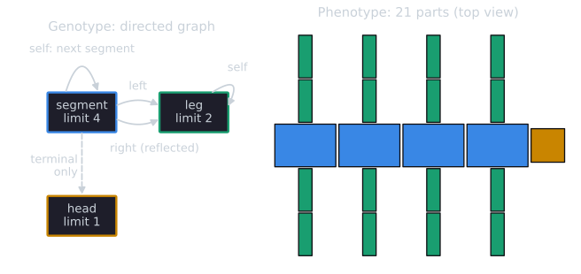
Three consequences follow from the encoding. A single mutation to the segment node changes all four segments at once, and a mutation to the recursive limit adds or removes a whole segment with its legs, which a direct list of 21 parts could not do in one step. Symmetry comes free from the reflected connection. And because each part carries a copy of its node's neurons, every duplicated segment or limb gets a similar but independent local control circuit, and connections between neurons in adjacent parts allow those circuits to be coordinated (Sims, 1994, §3.4). The same ideas, an indirect encoding that reuses one description many times, reappear in compositional pattern-producing networks.
Sims's creatures were never built, and some of what they did depended on the simulator. Early swimmers exploited integration error in the physics, and an early fitness measure for land locomotion rewarded creatures that simply fell over (Lehman et al., 2020); the surprising creativity of digital evolution tells these stories. His creatures also competed against each other for possession of a cube, which is discussed under competitive coevolution.
The reality gap
The difference between a controller's behavior in simulation and on the real robot is called the reality gap, the term in the title of Jakobi, Husbands and Harvey (1995). That paper tested a proposal that was then contested: that a carefully built simulation, with a proper treatment of noise, could produce controllers that work on real hardware. The authors built a simulation of a Khepera with infrared and ambient-light sensors, with empirically measured parameters, and evolved recurrent network controllers for obstacle avoidance and light seeking at three levels of noise: none, the noise level observed on the real robot, and twice that level. They then downloaded the evolved controllers onto the real Khepera.
The correspondence between simulated and real behavior depended on the noise. With realistic noise it was very close. Without noise, evolution found brittle strategies; one obstacle avoider circled the arena by always turning through exactly ninety degrees, which works only in a world that responds identically every time, and on the real robot it soon hit obstacles. With double noise, evolution exploited the noise itself: one light seeker approached the light in simulation only because random fluctuations occasionally pushed both of its sensors into an active band at once, and on the real robot it jittered in place. The authors concluded that simulation can work, for relatively simple robot-environment interactions, provided that the noise is at the right level, and they expected the approach to become harder as the interactions grew more complex.
Jakobi (1997) turned this into a design method, the minimal simulation. Instead of modelling everything accurately, which is rarely possible, the designer identifies a base set of robot-environment interactions sufficient for the desired behavior and models only those. Everything else in the simulation, the implementation aspects that exist only because some choice had to be made, is varied randomly from trial to trial, so that a controller can be reliably fit only by ignoring it. The base set aspects are varied too, so that reliably fit controllers must tolerate the inevitable differences between model and reality. Jakobi hypothesized that a simulation built this way can be inaccurate or incomplete and still produce controllers that transfer. He reported two sets of experiments with fast look-up-table simulations: a Khepera that solved a memory task in a T-maze, and the Sussex gantry robot, for which controllers evolved that told a triangle from a square under very noisy visual conditions and steered toward the triangle. In both, controllers that were reliably fit in simulation behaved robustly in reality.
Later work treated transfer as an objective in its own right. The transferability approach of Koos, Mouret and Doncieux (2013) optimizes fitness and a predicted simulation-to-reality disparity together with a multi-objective evolutionary algorithm, learning the disparity from a small number of tests on the real robot; on a navigation task with an e-puck robot and a walking task with an eight-degree-of-freedom quadruped, it found well-transferable controllers with about ten physical experiments.
A small experiment
The gap, and what noise does and does not do about it, can be seen in a toy. In tools/experiments/evolution/reality_gap.py in the site repository, a one-dimensional crawler has three point masses of 0.1 kg in a row, joined by two springs (stiffness 50 N/m, rest length 10 cm) whose rest lengths oscillate, like muscles that lengthen and shorten. The gait has four genes: the frequency $f$ (0.5 to 5 Hz), the two amplitudes (0 to 30% of the rest length), and the phase of the second spring relative to the first.
A body that only changes its shape moves forward only if the ground pushes it forward, and the simplest way to get that push is friction that resists sliding backward more than sliding forward. With the same friction in both directions, a stroke that is symmetric front to back, like the ones our crawler ends up using, gives back on the return whatever it gains. Snakes get direction-dependent friction from their belly scales: on a rough cloth, Hu, Nirody, Scott and Shelley (2009, Results and Fig. 1E) measured static friction coefficients of 0.11 for a snake sliding forward, 0.14 sliding backward and 0.20 sliding sideways, and in their model of slithering, equal coefficients in all directions gave little if any locomotion. Our crawler has a stronger asymmetry, as if it had backward-pointing bristles: a mass sliding forward feels a kinetic friction coefficient of 0.2, a mass sliding backward 0.8 (a smoothed Coulomb law). Fitness is steady progress, the mean velocity of the centre of mass between 2 s and 10 s of simulated time, which leaves out the start-up transient. A genetic algorithm with a population of 20, binary tournament selection, Gaussian mutation, elitism and no crossover runs for 40 generations. The script specifies every detail.
The evolved gaits walk, and every run found the same kind of gait. In all 30 runs in the nominal simulator, both amplitudes were at least 29.5% (against a maximum of 30%), the two springs were within 2 degrees of being in phase, and the frequency was between 3.50 and 3.61 Hz, with a median of 3.55 Hz. The frequency is not arbitrary. A chain of three equal masses $m$ joined by two equal springs $k$ can slide as a whole, and it has two modes of vibration, at $\frac{1}{2\pi}\sqrt{k/m} = 3.56$ Hz and $\frac{1}{2\pi}\sqrt{3k/m} = 6.16$ Hz. In the slower mode the two end masses move in opposite directions while the middle one stays still, which is exactly the motion that lengthening both springs together drives. Evolution found the resonance. Driven there, the springs swing well beyond their commanded range of 7 to 13 cm (after the start-up, a median gait's springs range from 0.7 to 19.3 cm, and since the toy does not model collisions, nothing stops neighbouring masses from coming that close), the end masses are flung forward and glide on the low forward friction, and the high backward friction holds them when the springs pull back. The result is fast for a toy, 115 cm/s, or about 32 cm per cycle for a body 20 cm long, and it is sustained: the same 30 gaits move at a median 117.6 cm/s between 10 s and 20 s. Friction is what makes it walk. With both coefficients set to 0.4, the same 30 gaits make no progress at all (a median of 0.000 cm/s).
The speed should not be read as a prediction for any real robot of this size. At resonance a spring pulls with up to about 4.7 N, six times the friction on a mass sliding backward and 24 times the friction on one sliding forward, and the end masses reach about 3.2 m/s. The crawler is a lightly damped oscillator driven at its natural frequency, with friction acting as a ratchet on its swing. Its speed is set by how large that swing can grow, and the toy has none of the limits that would cap it on hardware: no collisions between masses, no limit on actuator force or spring travel. What the toy does capture is the property the experiment needs, a gait whose performance depends sharply on parameters that the simulator gets slightly wrong.
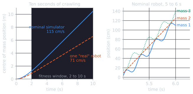
"Reality" is a fixed set of 100 robots, each with its own masses, friction coefficients and spring stiffness scaled by random factors (masses and stiffness by up to 25%, friction by up to 40%), and each with a 30 ms lag between the commanded and actual spring length, which the simulators do not model. Three simulators were used for evolution, 30 runs each: the nominal simulator; a noisy one that scores each genome by its mean over five robots with randomly perturbed masses, friction and stiffness, drawn afresh every generation, in the spirit of Jakobi, Husbands and Harvey (1995); and noisy+lag, which also draws a random actuator lag of up to 60 ms for each robot. Velocities in cm/s from 2 s to 10 s, as median [Q1, Q3] over 30 runs, rounded to 0.1 cm/s:
| Evolved in | Nominal simulator | Reality, mean of 100 robots | Reality, 10th percentile | Reality / simulator |
|---|---|---|---|---|
| Nominal | 115.1 [114.8, 115.1] | 70.2 [70.1, 70.2] | 42.5 [41.8, 42.9] | 0.61 [0.61, 0.61] |
| Noisy | 112.7 [108.4, 113.8] | 69.0 [67.9, 69.7] | 41.5 [39.3, 43.6] | 0.61 [0.61, 0.62] |
| Noisy + lag | 112.6 [108.5, 114.8] | 69.3 [68.0, 70.0] | 43.5 [41.0, 44.5] | 0.61 [0.61, 0.62] |
Our reading of these numbers is as follows. The gap is real and large: a gait evolved in the nominal simulator kept 61% of its simulated speed in "reality", and on the slowest tenth of the robots it managed about 42 cm/s. Both kinds of error contribute, and they compound. The parameter variation alone (the 100 robots without the lag) cut the median speed of the nominal gaits to 93.3 cm/s, and the lag alone (the nominal robot with the lag added) to 85.8 cm/s. Each detunes the resonance the gait relies on. A robot with stiffer springs or lighter masses resonates at a higher frequency, one with softer springs or heavier masses at a lower one, and either way it is no longer driven at its peak. A first-order lag of 30 ms passes a 3.55 Hz command with 83% of its amplitude, 34 degrees late, so the springs are driven less hard. The robots still crawl forward, every one of them (the slowest of the 3,000 pairs of a nominal gait and a "real" robot still made 16.5 cm/s), so here the gap is a loss of speed rather than a qualitative failure such as the ninety-degree turner's collisions.
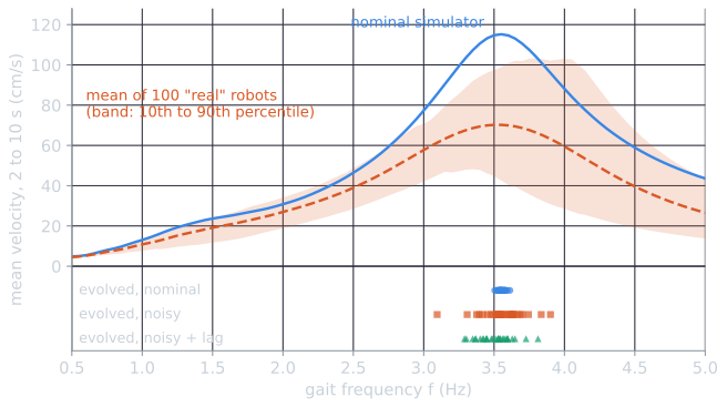
Noise did not close the gap, and in this toy it could not. Across the 900 pairs of a nominal run and a noisy run, the noisy gait did better in reality in 14% of pairs, and the median difference was 1.07 cm/s in favour of the nominal gait. With the lag inside the envelope of noise, the noisy gaits won 21% of pairs (a median difference of 0.84 cm/s in favour of the nominal gait), and their median 10th percentile, 43.5 cm/s against 42.5 cm/s, was higher by less than the spread between runs. The figure above shows why. The perturbed robots are spread on both sides of the nominal one, some resonating higher and some lower, so their mean speed still peaks at the nominal resonance: the gait that is best in the nominal simulator is also the best on average in reality, and there is nothing brittle for noise to steer evolution away from. What the noise did do was make each fitness evaluation less accurate, so the noisy runs settled less precisely on the gait (their frequencies ranged from 3.10 to 3.90 Hz and from 3.29 to 3.81 Hz, against 3.50 to 3.61 Hz for the nominal runs, and their phases strayed up to 24 degrees from in phase) and ended slightly slower.
This is consistent with Jakobi's account rather than a counterexample to it. Noise protects against controllers that exploit something the simulator offers and reality does not, such as a world that responds identically every time, which the exact ninety-degree turn depended on. Here the simulator is wrong about how fast the robot goes but right about which gait is best, so there is nothing of that kind to protect against, and the cost of noise remains: a noisy evaluation needs more trials to rank candidates reliably. For noise to pay off, the nominal optimum would have to be brittle, its performance collapsing under perturbations that a slightly worse gait survives. A four-gene gait with one smooth resonance peak has no such optimum, so the toy illustrates the gap, and the cost of the noise remedy, but not its benefit.
From simulation to fabrication
Lipson and Pollack (2000), in the GOLEM project, closed the loop between evolution and manufacture. Machines were assembled from bars, actuators and artificial neurons and evolved in a simulation of locomotion on a flat plane. The fittest designs, selected for their ability to move, were then produced by a rapid-prototyping machine that printed the thermoplastic body, after which the motors were attached by hand. The authors describe the result as autonomy of design and construction within a deliberately limited universe of parts; the evolved machines were simple, but they were the product of evolution in simulation followed by automatic fabrication.
Hiller and Lipson (2012) moved to soft materials. With multi-material 3-D printing, function can come from how hard and soft materials are distributed through a volume rather than from discrete parts. They used evolutionary algorithms first to design cantilever beams that bend into specified static profiles, whose printed versions matched predictions to within 0.5 to 7.6%, and then to design freeform soft robots that move forward using a volumetrically expanding actuator material. One such robot was fabricated and assembled, and its performance was confirmed with 15% error.
Voxel-based soft robots
A voxel representation, a three-dimensional grid in which each cell is empty or holds one of a few materials, makes soft bodies easy to encode and simulate. Cheney, MacCurdy, Clune and Lipson (2013) evolved such robots with four materials, two passive and two that expand and contract periodically in opposite phase, encoding each body with a compositional pattern-producing network evolved by NEAT. Selected for locomotion speed, CPPN-encoded robots moved faster than robots evolved with a direct voxel-by-voxel encoding, their shapes looked more natural, and performance rose as more materials were made available. Actuation was fixed by the material; only the body evolved.
Evolution Gym, or EvoGym (Bhatia et al., 2021), made voxel robots a standard benchmark. Its robots are two-dimensional grids of voxels, each empty, rigid, soft, or a horizontal or vertical actuator, simulated as mass-spring systems, and it offers more than 30 locomotion and manipulation tasks. Its baselines pair a body optimizer (a genetic algorithm, Bayesian optimization, or CPPN-NEAT) with reinforcement learning that trains a controller for each proposed body. The course's final project, coevolving soft robots with NEAT, used EvoGym's simplest walking task, and that article describes the benchmark in more detail.
Reconfigurable organisms built from cells
Kriegman, Blackiston, Levin and Bongard (2020) applied the same pipeline to living material. The building blocks were two kinds of voxel: passive, standing for skin tissue, and contractile, standing for heart muscle. An evolutionary algorithm searched, in a physics simulation, for arrangements that moved far in 10 simulated seconds; 100 independent runs were made for the locomotion goal. The best designs then passed through a robustness filter, which kept designs whose behavior survived random perturbations of their actuation, and a build filter, which removed designs that the current construction method could not produce or that were more than half muscle.
Selected designs were built by hand from cells of the frog Xenopus laevis. Pluripotent cells from blastula-stage embryos were aggregated and shaped by subtraction with microsurgery forceps and a cautery electrode, and cardiac progenitor cells were layered in where the design called for contraction. The resulting organisms, widely called xenobots, could move in water for days or weeks without added nutrients. The first pass through the pipeline produced designs with bounding gaits that spent on average 47% of each gait cycle off the ground, which the current build method could not produce in living tissue; adding first-order hydrodynamics and randomizing the phase of each contractile voxel in the simulator brought simulated behavior closer to what was observed. For the first design built, six organisms were made and observed for 10 minutes per trial; their direction of movement matched the simulated prediction ($p < 0.01$), and turning the design upside down significantly reduced displacement both in simulation and in the organisms. Other runs of the pipeline targeted object manipulation, object transport and collective behavior.
The result should be read precisely. The evolutionary search ran in simulation over a voxel model of two tissue types; the organisms were shaped by hand to approximate the evolved designs; cilia, which the model omitted, were suppressed by injecting messenger RNA so that only the heart tissue moved them; and the paper notes that some steps of the pipeline still require manual intervention. The organisms have no nervous system, and the transfer was demonstrated for at least one design in detail. What the paper shows is that a simulation-designed shape and tissue layout can produce a predicted direction of motion in a living aggregate of cells. It does not show general-purpose living machines.
Co-optimizing morphology and control
When both body and controller evolve, the two are coupled. A controller is tuned to the body it was evaluated with, so most mutations to the body make the robot worse until the controller readapts, and selection removes the changed bodies before that can happen. Cheney, Bongard, SunSpiral and Lipson (2018) argued that this coupling is a main reason body-brain co-optimization stalls in early local optima, and proposed morphological innovation protection: temporarily reducing the selection pressure on individuals whose bodies have just changed, giving subsequent controller mutations time to readapt. They reported that this helped avoid local optima, converged to similar highly fit body plans from widely varying initial conditions, and sustained fitness improvement later into optimization, while describing it as only a first step toward scalable co-optimization. The idea parallels the protection that speciation in NEAT gives to new network structure.
Embodied evolution
Another response to the reality gap is to evolve on the robots themselves, continuously, after deployment. Watson, Ficici and Pollack (2002) give the full account of embodied evolution, which the same group first presented in 1999, in which a population of physical robots runs a fully decentralized, asynchronous evolutionary algorithm. Each robot carries one controller, robots pass genetic material to nearby robots, and receiving it can replace part of a robot's own genome, in the manner of a microbial genetic algorithm (Bredeche, Haasdijk and Prieto, 2018); no central computer selects or evaluates. Their population was eight robots, and the task was phototaxis. Since the evaluations happen on the hardware and the controllers keep adapting after deployment, there is no simulator to bridge, at the price of the slow, noisy evaluations that simulation was introduced to avoid. A review by Bredeche, Haasdijk and Prieto (2018) traces a shift in this line of work from using small groups of robots (fewer than ten) as a parallel search method to using embodied evolution as an online, distributed way to learn collective behaviors in swarm-like groups. The algorithmic structure is that of the island and cellular models, with physical distance taking the place of a migration topology.
Open problems
Doncieux, Bredeche, Mouret and Eiben (2015) review the field's achievements and open issues, and several themes recur in the work above.
- Evaluation cost. Real evaluations are slow, and accurate simulations of soft, contact-rich or fluid environments are expensive. Quality-diversity methods, which precompute a repertoire of behaviors in simulation and then search it on the real robot, are one response; MAP-Elites and novelty search describes the damage-recovery experiments built on them.
- The fitness function. Every case above, from Sims's falling creatures to Jakobi's ninety-degree turns, shows evolution optimizing what was measured. The behaviors that matter on real hardware, such as robustness and energy use, must be measured or they will not be selected.
- Scale. Evolved robots remain simple compared with engineered ones, and the coupling between body and brain makes larger designs harder to evolve, not merely slower.
- The step to hardware. Each fabrication result above involved manual steps and a simplified model. That is not a criticism of the work, which reports these limits itself, but it marks the distance between evolving a design and evolving a working machine.
References
- Bhatia, J., Jackson, H., Tian, Y., Xu, J., and Matusik, W. (2021). Evolution Gym: A large-scale benchmark for evolving soft robots. In Advances in Neural Information Processing Systems 34, 2201–2214.
- Bredeche, N., Haasdijk, E., and Prieto, A. (2018). Embodied evolution in collective robotics: A review. Frontiers in Robotics and AI, 5, 12.
- Cheney, N., Bongard, J., SunSpiral, V., and Lipson, H. (2018). Scalable co-optimization of morphology and control in embodied machines. Journal of the Royal Society Interface, 15(143), 20170937.
- Cheney, N., MacCurdy, R., Clune, J., and Lipson, H. (2013). Unshackling evolution: Evolving soft robots with multiple materials and a powerful generative encoding. In Proceedings of the 15th Annual Conference on Genetic and Evolutionary Computation (GECCO '13), 167–174.
- Doncieux, S., Bredeche, N., Mouret, J.-B., and Eiben, A. E. (2015). Evolutionary robotics: What, why, and where to. Frontiers in Robotics and AI, 2, 4.
- Eiben, A. E., and Smith, J. E. (2015). Introduction to Evolutionary Computing, 2nd ed., chapter 17. Springer.
- Floreano, D., and Mondada, F. (1994). Automatic creation of an autonomous agent: Genetic evolution of a neural-network driven robot. In From Animals to Animats 3: Proceedings of the Third International Conference on Simulation of Adaptive Behavior, 421–430. MIT Press.
- Hiller, J., and Lipson, H. (2012). Automatic design and manufacture of soft robots. IEEE Transactions on Robotics, 28(2), 457–466.
- Hu, D. L., Nirody, J., Scott, T., and Shelley, M. J. (2009). The mechanics of slithering locomotion. Proceedings of the National Academy of Sciences, 106(25), 10081–10085.
- Jakobi, N. (1997). Evolutionary robotics and the radical envelope-of-noise hypothesis. Adaptive Behavior, 6(2), 325–368.
- Jakobi, N., Husbands, P., and Harvey, I. (1995). Noise and the reality gap: The use of simulation in evolutionary robotics. In Advances in Artificial Life (ECAL '95), Lecture Notes in Computer Science 929, 704–720. Springer.
- Koos, S., Mouret, J.-B., and Doncieux, S. (2013). The transferability approach: Crossing the reality gap in evolutionary robotics. IEEE Transactions on Evolutionary Computation, 17(1), 122–145.
- Kriegman, S., Blackiston, D., Levin, M., and Bongard, J. (2020). A scalable pipeline for designing reconfigurable organisms. Proceedings of the National Academy of Sciences, 117(4), 1853–1859.
- Lehman, J., et al. (2020). The surprising creativity of digital evolution: A collection of anecdotes from the evolutionary computation and artificial life research communities. Artificial Life, 26(2), 274–306.
- Lipson, H., and Pollack, J. B. (2000). Automatic design and manufacture of robotic lifeforms. Nature, 406(6799), 974–978.
- Nolfi, S., and Floreano, D. (2000). Evolutionary Robotics: The Biology, Intelligence, and Technology of Self-Organizing Machines. MIT Press.
- Sims, K. (1994). Evolving virtual creatures. In Proceedings of the 21st Annual Conference on Computer Graphics and Interactive Techniques (SIGGRAPH '94), 15–22.
- Watson, R. A., Ficici, S. G., and Pollack, J. B. (2002). Embodied evolution: Distributing an evolutionary algorithm in a population of robots. Robotics and Autonomous Systems, 39(1), 1–18.