Consider minimizing a function of 20 variables with a genetic algorithm that encodes each variable in 16 bits. The standard approach evolves one population of 320-bit chromosomes, and every change to one variable is judged together with the current values of the other 19. An alternative is to give each variable its own population of 16-bit chromosomes, evolve the 20 populations separately, and judge a candidate value for one variable by plugging it into a complete solution assembled from good values of the others. On the Rastrigin function, a standard multimodal test problem, the second approach found the best point that the 16-bit encoding can represent in at least three quarters of 30 runs, while the first was still far from the optimum after the same 100,000 evaluations. Rotate the same function, so that the variables no longer act independently, and the ranking reverses.
The second approach is cooperative coevolution: a problem is decomposed into parts, each part evolves in its own population (a species), and individuals are rewarded for how well they work with the members of the other species. Where competitive coevolution scores an individual by contests against other evolving individuals, cooperative coevolution scores it by its contribution to a joint solution. Both make fitness relative: an individual's score depends on which members of other populations it is evaluated with, and changes as they evolve. This article covers the architecture, the choices it forces, a pathology called relative overgeneralization, its use for optimization in thousands of dimensions, and its role in evolving neural networks. Eiben and Smith (2015, ch. 15) give a short textbook treatment.
The architecture
Potter and De Jong (1994) proposed the cooperative coevolutionary genetic algorithm (CCGA) with these elements: a species represents a subcomponent of a solution; complete solutions are assembled from representative members of each species; an individual's credit is the fitness of the complete solutions it takes part in; each species is evolved by a standard genetic algorithm; and, when needed, the number of species should itself evolve. Species are genetically isolated, mating only within their own population, and interact only through evaluation.
For function optimization the decomposition is given: one species per variable. Their first algorithm, CCGA-1, works as follows.
- Initialize one population per variable. Evaluate each individual by combining it with a randomly chosen individual from each of the other species.
- Evolve the species in turn, round robin. For the current species, apply selection, crossover and mutation as in an ordinary GA, and evaluate each new individual by combining it with the current best individual of every other species, which are held fixed while this species is evaluated.
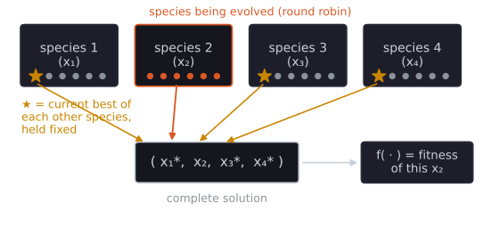
Potter and De Jong called this the simplest form of credit assignment imaginable, and noted its resemblance to numerical methods that optimize one variable at a time while holding the others fixed, which work well when the variables are reasonably independent and poorly when they interact.
They compared CCGA-1 with a standard GA that differed only in using a single population: 16 bits per variable, fitness-proportional selection with a scaling window, elitism, two-point crossover, mutation at one over the chromosome length, populations of 100, and 100,000 evaluations, averaged over 50 runs. On four multimodal functions, Rastrigin (20 variables), Schwefel (10), Griewangk (10) and Ackley (30), CCGA-1 was significantly better in both final value and speed. Its advantage was smallest on Griewangk, whose product term couples the variables. On the two-variable Rosenbrock function, whose curved valley couples the variables strongly, CCGA-1 did much worse than the GA. They attributed this to the greedy credit assignment and tried a second version, CCGA-2, which evaluates each new individual twice, once with the best members of the other species and once with randomly chosen members, and keeps the better result. CCGA-2 matched the GA on Rosenbrock, at the cost of slightly worse performance than CCGA-1 on Rastrigin. There was also a computational bonus: decoding a 16-bit chromosome is cheaper than decoding a full one, and on the 30-variable Ackley function the standard GA took about six times as long for the same number of evaluations.
Potter and De Jong (2000) developed the general architecture further. Credit assignment works at two levels. Within a species, the representatives of the other species are fixed during evaluation, so an individual's fitness differs from its rivals' only through its own contribution, and no attempt is made to divide credit among species. At the level of species, a species whose members contribute too little is removed. When the best collaboration stops improving by a set amount within a set number of generations, a new, randomly initialized species is added, so that both the number of species and their roles can emerge. On a string-matching task they showed that the species came to cover different niches of the target set, with an appropriate number of species; they then applied the architecture to growing cascade neural networks, adding a species for each new hidden unit. Because species interact only through occasional exchange of representatives, the architecture parallelizes naturally, much as island models do, and different species can use different representations.
Separable and non-separable problems
A function is separable if it can be optimized one variable at a time: the best value of each variable does not depend on the values of the others. Rastrigin's function,
$$f(\mathbf{x}) = 10n + \sum_{i=1}^{n} \left( x_i^2 - 10 \cos(2 \pi x_i) \right),$$
is a sum of one-variable terms, so it is separable however many local minima it has (one near each integer point of the box $[-5.12, 5.12]^n$, $11^n$ in all). Rotating the coordinate system, $f(R\mathbf{x})$ for an orthogonal matrix $R$, leaves the shape of the function unchanged but mixes every variable into every term, so it is no longer separable. Rosenbrock's function,
$$f(\mathbf{x}) = \sum_{i=1}^{n-1} \left[ 100 (x_{i+1} - x_i^2)^2 + (1 - x_i)^2 \right],$$
couples each variable to its neighbours.
Two dimensions show why separability matters to an algorithm that changes one variable at a time. Strip CCGA-1 down to its logic: let each species be a perfect optimizer of its own variable, so that a species step replaces $x_1$ by the value that minimizes $f$ with $x_2$ held at its current value, and the next step does the same for $x_2$. This is coordinate-wise best response, the idealized limit of the round-robin scheme. For a separable function the best $x_1$ does not depend on $x_2$ at all, because $f(x_1, x_2) = g(x_1) + h(x_2)$ and the term $h(x_2)$ is a constant while $x_1$ is being chosen. So one sweep finds the global minimum from any starting point. Rotating the function by 30° breaks this: the value of $x_1$ that is best depends on where $x_2$ is, and each species can only move along its own axis.
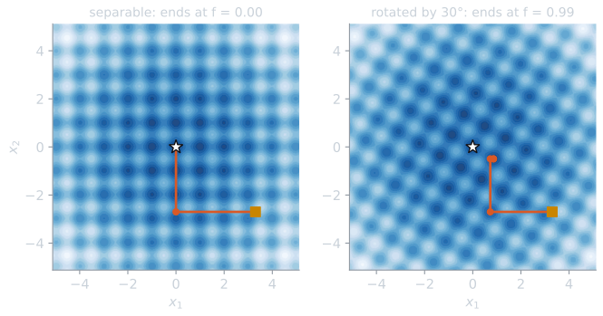
The steps from $(3.3, -2.7)$, computed on a grid of step 0.0005 by tools/experiments/evolution/cooperative_examples.py: on the separable function, $(3.3, -2.7) \to (0, -2.7) \to (0, 0)$, with $f = 0$. On the rotated function, $(3.3, -2.7) \to (0.728, -2.7) \to (0.728, -0.493) \to (0.861, -0.493) \to (0.861, -0.498)$, after which neither variable can move, with $f = 0.995$. From 1,000 random starting points in the box, best response reached the global minimum every time on the separable function and 11.2% of the time on the rotated one, with a median final value of 1.990 (quartiles 0.995 and 3.980). The point where it stops is a Nash equilibrium of the game in which each variable is a player minimizing the same $f$: no player can do better by changing its own move alone. An algorithm that evaluates each variable against the best values of the others can come to rest at such points, and on a non-separable function many of them are not the optimum.
The script tools/experiments/evolution/cooperative_coevolution.py in the site repository compares a GA, CCGA-1 and CCGA-2 on these three functions with 100,000 evaluations each. The settings follow Potter and De Jong with three changes: binary tournament selection in place of fitness-proportional selection with a scaling window, the standard constant 10 in Rastrigin's function where they used 3, and 10 variables for Rosenbrock's function where they used 2. Rastrigin's function has 20 variables, as in their study, and the rotated version is our addition. The best value found, median and interquartile range over 30 seeded runs:
| Function | GA | CCGA-1 | CCGA-2 |
|---|---|---|---|
| Rastrigin, separable | 12.23 [9.71, 15.22] | $2.42 \times 10^{-5}$ [$2.42 \times 10^{-5}$, $2.42 \times 10^{-5}$] | $1.02 \times 10^{-4}$ [$7.27 \times 10^{-5}$, $2.42 \times 10^{-4}$] |
| Rastrigin, rotated | 54.29 [47.78, 63.86] | 109.4 [98.75, 134.1] | 107.5 [96.26, 115.9] |
| Rosenbrock, 10 variables | 8.15 [7.60, 8.95] | 3.25 [1.88, 6.47] | 4.00 [0.46, 6.64] |
On the separable function, CCGA-1 reached $2.42 \times 10^{-5}$ in at least three quarters of the runs, which is the optimum of the 16-bit grid: no 16-bit value lies exactly at 0, and the nearest, $x_i \approx -7.8 \times 10^{-5}$, contributes $1.2 \times 10^{-6}$ per variable. Both coevolutionary versions ended below the GA in all 30 runs, and after 10,000 evaluations CCGA-1 was already at 1.56 against the GA's 28.9. Rotation reversed the result: the GA's median more than quadrupled, from 12 to 54, while both coevolutionary versions ended near 108, and each beat the GA in only 1 of 30 runs. A species controls one coordinate and can move only along that axis, and after rotation no axis is a direction along which the function can be optimized on its own.
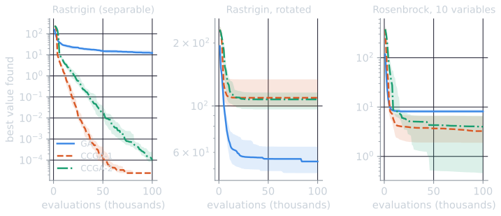
The curves show when the outcome is decided. On the rotated function both coevolutionary versions had essentially stopped by 10,000 evaluations (CCGA-1's median was 110.9 then and 109.4 at the end), in the way the two-dimensional best-response example stopped at its first point where no single-axis move helped. The GA, which changes all coordinates at once through crossover and mutation, kept improving, from a median of 68.4 at 10,000 evaluations to 55.9 at 50,000 and 54.3 at the end.
Rosenbrock's function did not reproduce Potter and De Jong's result. In this setup CCGA-1 ended below the GA in 29 of 30 runs and CCGA-2 in 27, so the interaction between neighbouring variables, though real, did not defeat the coevolutionary versions. The experiment differs from theirs in dimension (10 variables rather than 2) and in selection, and the GA itself stalled near 8. The comparison illustrates a point Wiegand (2003) argued at length: whether a problem is separable does not by itself determine whether cooperative coevolution helps. What matters is the kind of interaction.
Collaborators and credit
Every cooperative coevolutionary algorithm must decide which members of the other species an individual is evaluated with, and how to turn several evaluations into one fitness value. CCGA-1 uses one collaborator per species, the current best; CCGA-2 uses two, the best and a random one, and takes the better result. Wiegand, Liles and De Jong (2001) studied these choices empirically, and Wiegand (2003) describes them as three attributes of a collaboration method:
- Sample size: how many collaborators from each other species. Each one costs an evaluation, and with several species the costs multiply.
- Selective bias: how collaborators are chosen, from uniformly at random to always the best.
- Credit assignment: how the results are combined, optimistic (the maximum), hedge (the mean) or pessimistic (the minimum).
On constructed test problems, Wiegand (2003) found that a single collaborator was best when the interactions between variables did not cross the boundaries between populations, and that more collaborators helped when they did, specifically when the effect of a change to one population's part could not be predicted in sign or magnitude from the parts alone. Increasing the sample size helped more than biasing it toward the best, which he noted agrees with the earlier study, and for static optimization, optimistic credit assignment was typically a good choice.
Relative overgeneralization
Optimistic credit assignment also counters a problem that goes beyond sampling noise: cooperative coevolution is not, in general, an optimizer. Wiegand (2003) calls the problem relative overgeneralization: populations are attracted toward regions of the search space where many strategies perform well relative to the individuals they are paired with, which may be far from the optimum.
The climbing game of Claus and Boutilier (1998), a test problem from multiagent reinforcement learning, shows the effect. Two agents each choose one of three actions, and both receive the same payoff for the joint action (as used by Panait, Luke and Wiegand, 2006):
| $b = 0$ | $b = 1$ | $b = 2$ | |
|---|---|---|---|
| $a = 0$ | 11 | $-30$ | 0 |
| $a = 1$ | $-30$ | 7 | 6 |
| $a = 2$ | 0 | 0 | 5 |
The best joint action is $(0, 0)$, worth 11. But an agent that tries action 0 against a partner who chooses at random gets $(11 - 30 + 0)/3 = -6.33$ on average; action 1 gets $-5.67$ and action 2 gets $1.67$. Judged by average performance with whatever partners the other population currently holds, the optimal action looks worst, because it is punished heavily whenever the partner is not also optimal. The safe actions, which do moderately well with any partner, are the "jack-of-all-trades" choices that Panait, Luke and Wiegand (2006) describe the populations being drawn to. They stress that this is not the local-optimum problem of ordinary search, nor sampling error: in their analysis, even with infinite populations and no variation operators, the coevolutionary dynamics are not necessarily attracted to the optimum, whereas a GA under the same conditions would be attracted to the unique maximum. Their remedy biases each individual's fitness toward an estimate of the payoff it would receive with its ideal collaborator, weighting the two parts with a parameter $\delta$.
The same effect appears with continuous actions, where it is easier to see. Take two agents choosing $x$ and $y$ in $[0, 1]$, with a joint payoff of our own construction that has a tall, narrow peak of height 10 at $(0.8, 0.8)$ and a broad hill of height 6 centred at $(0.25, 0.25)$ (Gaussians of standard deviation 0.05 and 0.25; the payoff is the larger of the two). An agent's action $x$ can be credited in two ways. Hedge credit averages the payoff over partners spread uniformly across $[0, 1]$; optimistic credit takes the payoff with the best partner. Computed on a grid of 1,001 points by cooperative_examples.py:
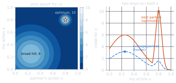
Averaged over partners, the credit is highest at $x = 0.25$ (3.16), and the optimal action $x = 0.8$ earns only 1.51, because it pays well only with a partner within a few hundredths of 0.8. With the best partner, $x = 0.8$ earns 10 and $x = 0.25$ earns 6. A population of agents credited by averages climbs the broad hill: each action is judged by how it does with typical partners, and typical partners favour the robust choice. This is relative overgeneralization in a picture.
The dynamics of the climbing game can also be followed exactly, without sampling, by treating both populations as infinitely large. Each action's fitness is its expected payoff against the other population's current mixture; binary tournament selection then gives action $a$ the share $p_a^2 + 2p_a \sum_{c:\, f_c < f_a} p_c$ (it is selected when both draws are $a$, or when one is $a$ and the other a less fit action; no two actions tie here), and mutation at rate 0.05 replaces a share 0.05 of each population with uniformly random actions. The payoff table is not symmetric (row action 1 against column action 2 pays 6, but row action 2 against column action 1 pays 0), so the row population $A$ and the column population $B$ take different paths. Starting from equal shares (computed by cooperative_examples.py, three decimals for shares, two for fitness):
| Generation | $A$: shares of actions 0, 1, 2 | $A$: fitness | $B$: shares of actions 0, 1, 2 | $B$: fitness |
|---|---|---|---|---|
| 0 | 0.333, 0.333, 0.333 | −6.33, −5.67, 1.67 | 0.333, 0.333, 0.333 | −6.33, −7.67, 3.67 |
| 1 | 0.122, 0.333, 0.544 | 0.00, −5.88, 2.72 | 0.333, 0.122, 0.544 | −8.66, −1.33, 4.72 |
| 2 | 0.108, 0.122, 0.770 | −1.90, 1.71, 3.85 | 0.122, 0.108, 0.770 | −2.48, −2.39, 4.58 |
| 4 | 0.017, 0.120, 0.863 | −0.48, 5.39, 4.80 | 0.018, 0.022, 0.960 | −3.41, 0.32, 5.03 |
| 6 | 0.017, 0.405, 0.578 | −0.34, 5.41, 4.83 | 0.017, 0.018, 0.966 | −11.97, 2.33, 5.32 |
| 8 | 0.017, 0.837, 0.146 | −0.34, 5.41, 4.83 | 0.017, 0.018, 0.966 | −24.92, 5.35, 5.75 |
| 10 | 0.017, 0.963, 0.020 | −1.30, 5.44, 4.67 | 0.017, 0.050, 0.933 | −28.72, 6.24, 5.88 |
| 12 | 0.017, 0.966, 0.018 | −6.17, 5.60, 3.86 | 0.017, 0.212, 0.771 | −28.78, 6.25, 5.88 |
| 14 | 0.017, 0.966, 0.018 | −17.74, 5.99, 1.93 | 0.017, 0.598, 0.385 | −28.78, 6.25, 5.88 |
| 17 | 0.017, 0.966, 0.018 | −28.69, 6.35, 0.10 | 0.017, 0.962, 0.021 | −28.78, 6.25, 5.88 |
Action 2 is the best reply to a uniform partner in both populations and holds 77% of each by generation 2, while action 0, the optimum, falls to the floor of about 0.017 that mutation provides by generation 4. From there the two populations take turns. With $B$ playing mostly 2, $A$'s action 1 earns more than its action 2 (5.39 against 4.80 at generation 4), and $A$ moves to action 1 by generation 10. $B$'s action 2 stays best while $A$ still plays 2, because column action 1 earns 0 against it; once $A$ plays 1, $B$'s action 1 earns 7 against action 2's 6, and $B$ follows by generation 17. Both settle on $(1, 1)$, payoff 7, and action 0, punished by the $-30$ against action 1, never recovers. With optimistic credit, the expected best of five random partners, the same calculation sends action 0 to 0.966 of both populations by generation 6: at the start its expected best payoff in $A$ is 9.43 against 6.72 and 4.34, and the advantage only grows as partners learn to play it.
The second part of cooperative_coevolution.py runs two populations of 20 agents on this game, each individual being one action, for 50 generations with binary tournament selection and a mutation rate of 0.05, under five collaboration schemes. The number of the 30 runs ending with each joint action held by a majority of both populations:
| Scheme | $(0, 0)$, payoff 11 | $(1, 1)$, payoff 7 | $(2, 2)$, payoff 5 | $(1, 2)$, payoff 6 |
|---|---|---|---|---|
| Best of the other population | 5 | 25 | 0 | 0 |
| One random partner | 9 | 21 | 0 | 0 |
| Average over the whole population | 3 | 19 | 1 | 7 |
| Best and one random, maximum | 28 | 2 | 0 | 0 |
| Maximum over 5 random partners | 28 | 2 | 0 | 0 |
Averaging over the entire partner population, the most thorough evaluation of the five, found the optimum least often. The populations usually settled on $(1, 1)$. The payoffs suggest why: action 2 does best against a random partner and spreads first; once partners mostly play 2, action 1 earns 6 against them where action 2 earns 5, so action 1 takes over; and action 0 stays unattractive because it pays $-30$ against action 1. The two optimistic schemes, which credit an individual with its best result, found $(0, 0)$ in 28 of 30 runs. Weakening the penalty helps averaging: with $-30$ replaced by $-20$, $-10$, $-5$ and $0$, it found the optimum in 5, 6, 8 and 15 runs, while the optimistic scheme found it in 28 every time. Choosing the best collaborator from the previous generation, close to what CCGA-1 does, is not optimistic in this sense, and it found the optimum in only 5 runs.
Large-scale optimization
Cooperative coevolution returned to prominence as a way to optimize functions of hundreds or thousands of variables, where standard evolutionary algorithms degrade. The difficulty is the decomposition. One species per variable fails on non-separable functions, and the variable interactions are rarely known in advance.
Yang, Tang and Yao (2008) proposed random grouping. The $n$ variables are split at random into $m$ groups of $s = n/m$ variables each, each group is optimized in turn by a differential evolution algorithm for a fixed budget, and the split is redrawn at the start of every cycle. Two interacting variables are not kept apart permanently; in each cycle they share a group with probability $1/m$. They showed that over $N$ cycles the probability that the two share a group in at least $k$ of them is
$$P_k = \sum_{r=k}^{N} \binom{N}{r} \left( \frac{1}{m} \right)^{r} \left( 1 - \frac{1}{m} \right)^{N - r}.$$
For $n = 1000$ variables in $m = 10$ groups of 100 and $N = 50$ cycles, $P_1 = 1 - 0.9^{50} = 0.9948$ and $P_2 = 0.9662$. Their algorithm, DECC-G, also used adaptive weighting, which after each cycle evolves a vector of weights, one per group, that scale each group's variables together, and it was tested on benchmark functions of up to 1,000 variables. The calculation covers a pair of variables. For a group of $v$ interacting variables, all $v$ land together with probability $(1/m)^{v-1}$ per cycle; with $v = 5$ and $m = 10$ that is $10^{-4}$, and over 50 cycles the chance of it happening even once is about 0.5% (our calculation).
Omidvar, Li, Mei and Yao (2014) proposed instead to find the interactions before optimizing. Differential grouping rests on a simple test. Perturb variable $x_i$ by $\delta$ and record the change in $f$; then set another variable $x_j$ to a different value and repeat. If the two changes differ, $x_i$ and $x_j$ interact. For $f(x_1, x_2) = x_1^2 + x_1 x_2 + x_2^2$ with $\delta = 1$, the change is $f(1, 0) - f(0, 0) = 1$ at $x_2 = 0$, but $f(1, 1) - f(0, 1) = 3 - 1 = 2$ at $x_2 = 1$, so the variables interact. For $x_1^2 + x_2^2$ both changes are 1. The algorithm applies the test to pairs of variables, with a threshold $\epsilon = 10^{-3}$ on the difference, and puts each variable that interacts with $x_i$ into $x_i$'s group. The cost depends on the structure it finds: for 1,000 variables, 21,000 evaluations if they form 20 groups of 50, but 1,001,000 if the function is fully separable, since then every pair must be tested. On the 20 functions of the CEC 2010 large-scale benchmark, all with 1,000 variables, it grouped the interacting variables perfectly on 13 functions and had low accuracy on almost all the variants of Rosenbrock's function, which the authors left for further study.
Neuroevolution
Neural networks offer a natural decomposition into neurons, and cooperative coevolution became an important approach in neuroevolution. SANE (Symbiotic Adaptive Neuro-Evolution) evolves a single population of neurons instead of a population of networks: networks are assembled from neurons, and each neuron's fitness depends on the performance of the networks it took part in (Moriarty and Miikkulainen, 1996). Potter and De Jong (2000) point out that rewarding neurons for how well they collaborate maintains diversity in the population and produces a form of emergent decomposition. In a later version, as they describe it, a second population of network blueprints records combinations of neurons that work well together, and a neuron's fitness is the average of the five best networks it took part in.
ESP (Enforced Subpopulations) makes the decomposition explicit: one subpopulation for each hidden-unit position, with neurons recombined only within their own subpopulation, and each network built from one neuron of each. Gomez and Miikkulainen (1997) introduced it to evolve networks with memory, and combined it with incremental evolution on a prey-capture task, evaluating the population first on easier versions of the task and then on harder ones. In ESP the species are positions in a fixed architecture; NEAT instead evolves whole networks and uses species to protect new structure, a different use of the word.
Where cooperative coevolution fits
Cooperative coevolution pays off when a problem decomposes into parts that interact weakly or in predictable ways: separable and partially separable functions, teams of agents with distinct roles, networks of specialized units. It shrinks each population's search space, parallelizes naturally, and allows different representations for different parts. Its costs are the decomposition, which is either supplied by hand or must be learned at a price in evaluations, and the relative fitness, which can favour robust partners over optimal ones. The separable and rotated versions of Rastrigin's function, identical in shape and opposite in outcome, show both sides.
References
- Claus, C., and Boutilier, C. (1998). The dynamics of reinforcement learning in cooperative multiagent systems. In Proceedings of the Fifteenth National Conference on Artificial Intelligence (AAAI-98), 746–752. AAAI Press.
- Eiben, A. E., and Smith, J. E. (2015). Introduction to Evolutionary Computing, 2nd ed., chapter 15. Springer.
- Gomez, F., and Miikkulainen, R. (1997). Incremental evolution of complex general behavior. Adaptive Behavior, 5(3–4), 317–342.
- Moriarty, D. E., and Miikkulainen, R. (1996). Efficient reinforcement learning through symbiotic evolution. Machine Learning, 22(1–3), 11–32.
- Omidvar, M. N., Li, X., Mei, Y., and Yao, X. (2014). Cooperative co-evolution with differential grouping for large scale optimization. IEEE Transactions on Evolutionary Computation, 18(3), 378–393.
- Panait, L., Luke, S., and Wiegand, R. P. (2006). Biasing coevolutionary search for optimal multiagent behaviors. IEEE Transactions on Evolutionary Computation, 10(6), 629–645.
- Potter, M. A., and De Jong, K. A. (1994). A cooperative coevolutionary approach to function optimization. In Y. Davidor, H.-P. Schwefel and R. Männer (eds.), Parallel Problem Solving from Nature: PPSN III, Lecture Notes in Computer Science 866, 249–257. Springer.
- Potter, M. A., and De Jong, K. A. (2000). Cooperative coevolution: An architecture for evolving coadapted subcomponents. Evolutionary Computation, 8(1), 1–29.
- Wiegand, R. P. (2003). An Analysis of Cooperative Coevolutionary Algorithms. Doctoral dissertation, George Mason University.
- Wiegand, R. P., Liles, W. C., and De Jong, K. A. (2001). An empirical analysis of collaboration methods in cooperative coevolutionary algorithms. In L. Spector et al. (eds.), Proceedings of the Genetic and Evolutionary Computation Conference (GECCO-2001), 1235–1242. Morgan Kaufmann.
- Yang, Z., Tang, K., and Yao, X. (2008). Large scale evolutionary optimization using cooperative coevolution. Information Sciences, 178(15), 2985–2999.