Suppose the goal is to evolve a program that plays checkers. A standard evolutionary algorithm needs a fitness function, and the obvious one is a score against a strong existing program. It fails at once: a population of random players loses every game against a strong opponent, every individual gets the same score, and selection has nothing to act on. A weak fixed opponent has the opposite problem. Once the population beats it, the score again stops distinguishing good from better. What the population needs is an opponent pitched at its own level, one that improves as it does. The population itself is such an opponent.
In competitive coevolution, an individual's fitness is the outcome of contests with other individuals that are evolving at the same time: members of its own population, or of a second population whose success is defined as the first one's failure. The idea removes the need for a hand-made fitness function where none is available or any fixed one is too hard or too easy, and it introduces problems that an ordinary evolutionary algorithm never has. Cooperative coevolution treats the other main form, in which populations are rewarded for working together, and Red Queen dynamics treats the arms races and cycles that coevolution produces. Eiben and Smith (2015, ch. 15) give a short textbook treatment of both forms.
Absolute and relative fitness
In a standard evolutionary algorithm, fitness is absolute (also called objective or external): a function of the individual alone, which gives the same value whenever and wherever it is evaluated. In coevolution, fitness is relative (also called subjective or internal): it depends on which other individuals the individual meets, and those change every generation. Three consequences follow.
- Scores are not comparable across generations. A player that wins 60% of its games in generation 100 may be much stronger than one that won 90% in generation 10, because its opponents are stronger. A rising score can also mean that the opponents have become weaker, and a flat score can hide steady improvement on both sides.
- The ordering can be intransitive. If $A$ beats $B$, $B$ beats $C$ and $C$ beats $A$, as in rock-paper-scissors, there is no best individual, and a population can cycle through the three indefinitely while every generation's winners look like progress.
- The gradient can disappear. If one side becomes much stronger than the other, every contest has the same outcome, all individuals on both sides receive equal fitness, and selection becomes random, the same failure as the fixed strong opponent in the checkers example.
Coevolutionary systems come in two arrangements. In a one-population system, individuals of the same kind compete with each other, as players of a symmetric game do. In a two-population system, the populations play different roles: solutions and the tests that try to break them, predators and prey, or the two sides of an asymmetric game. Rosin and Belew (1995) call the individual being evaluated the host and the individuals evaluating it the parasites; in a two-population system each population takes both roles in turn. Biologists call selection of this kind, in which the value of a trait depends on how common other traits are, frequency-dependent selection. Natural selection for computer scientists notes that a standard evolutionary algorithm leaves out the moving environment that coevolution restores.
Hillis's sorting networks
An early and widely cited demonstration that coevolution can improve an optimizer came from Danny Hillis (1990), on a problem with a long history. A sorting network sorts $n$ numbers with a fixed sequence of compare-exchange operations, each of which compares the values on two lines and swaps them if they are out of order. For 16 inputs, Bose and Nelson gave a 65-comparator network in 1962. Batcher, and independently Floyd and Knuth, reduced this to 63 in 1964; Shapiro found 62 in 1969, and Green found 60 later the same year. Hillis cites Green's 60 as the best known.
A small network shows how the operations work. The network below sorts four inputs with five comparators. Each vertical bar compares the values on its two wires and leaves the smaller on the upper wire. Following the input $(3, 1, 4, 2)$ from left to right: the first comparator swaps 3 and 1, giving $(1, 3, 4, 2)$; the second swaps 4 and 2, giving $(1, 3, 2, 4)$; the third and fourth find their pairs already in order; and the last swaps the middle two, giving $(1, 2, 3, 4)$. The sequence of comparators is fixed in advance and does not depend on the data, which is what makes such networks attractive in hardware, and what makes them a natural genome: a list of wire pairs.
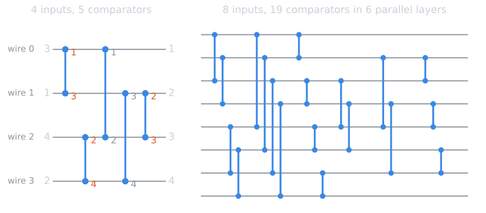
A network can be checked exactly, because of the 0-1 principle: a comparator network sorts every input if and only if it sorts all $2^{n}$ sequences of zeros and ones, 65,536 for 16 inputs rather than $16!$, about $2 \times 10^{13}$, permutations. The reason is that a comparator commutes with any non-decreasing function $g$ applied to every value: comparing $g(a)$ and $g(b)$ puts $g(\min(a, b))$ on the upper wire and $g(\max(a, b))$ on the lower. If a network leaves some input unsorted, with a larger value $x$ above a smaller $y$ on its output wires, then thresholding every value at $y$ (1 if greater than $y$, 0 otherwise) gives a binary input whose output has a 1 above a 0, so the network also fails on that binary input. Removing the last comparator of the four-input network illustrates it. The shortened network fails 16 of the 24 permutations, every one of them leaving $(1, 3, 2, 4)$, and it fails exactly the four binary inputs 0101, 0110, 1001 and 1010, each producing 0101. Thresholding the failed output $(1, 3, 2, 4)$ at 2 gives 0101 (these examples are computed by tools/experiments/evolution/competitive_examples.py).
Hillis evolved candidate networks, scoring each by the fraction of test inputs it sorted, in populations of 65,536 individuals on a Connection Machine, for up to 5,000 generations. The genotype was diploid, so a network had between 60 and 120 comparators; individuals lived on a two-dimensional toroidal grid and mated with nearby individuals; the better half survived each generation (truncation selection at 50%). Because most known minimal 16-input networks begin with the same 32 comparators, the initial population was homozygous for those 32, with the rest random. The search therefore began from the shared first half of the known solutions, a detail that matters when reading the result.
Without coevolution, the best networks found had 65 comparators, no better than Bose and Nelson's. Hillis identified two sources of waste. Populations converged on a few local optima and stopped there, and after the first generations most randomly chosen test cases were sorted correctly by almost every network, so they no longer distinguished good networks from bad ones.
His remedy was a second population. Hosts were sorting networks; parasites were sets of 10 to 20 test sequences. Both evolved on the same grid, and each network was scored on the tests of the parasite at its location. A parasite's score was the number of its tests the network failed, so the two fitness functions were exactly complementary. Hillis argued that the parasites helped in two ways. A large subpopulation sharing the same flaw became a target that parasites evolved to exploit, which kept the hosts from settling on one imperfect design, and since only tests that exposed weaknesses spread, a few tests per individual sufficed. The runs with parasites produced consistently better results, and the best network had 61 comparators: better than the networks of Batcher and Shapiro and than the 65 found without parasites, but one comparator more than Green's 60.
Axelrod and the prisoner's dilemma
Robert Axelrod's work on the iterated prisoner's dilemma is the other early landmark, from political science rather than computing. In each round two players simultaneously cooperate or defect. Mutual cooperation pays each 3, mutual defection 1, and a defector facing a cooperator receives 5 while the cooperator receives 0. In a single round defection is always the better reply, but over many rounds two players who cooperate do better than two who defect.
| Opponent cooperates | Opponent defects | |
|---|---|---|
| Cooperate | 3 | 0 |
| Defect | 5 | 1 |
(Payoff to the row player.) Whatever the opponent does, defecting pays 2 more than cooperating against a cooperator and 1 more against a defector, which is why a single round has defection as its only equilibrium. Repetition changes this, because a player's moves can now depend on what the other did before. Tit for tat cooperates on the first move and then copies the opponent's previous move. Against a player who always defects, it is exploited exactly once: over five rounds the moves are CDDDD against DDDDD, and the scores 4 against 9. Against itself, it cooperates throughout and earns 3 per round.
Axelrod (1980a) invited game theorists to submit strategies to a round-robin computer tournament. The 14 entries and a random strategy played each other, and the winner was the simplest entry, tit for tat, submitted by Anatol Rapoport: cooperate on the first move, then copy the opponent's previous move. A second tournament drew 62 entries from six countries, and tit for tat, again submitted by Rapoport, won again (Axelrod, 1980b). A strategy's tournament score is relative fitness in its plainest form.
Axelrod then let a genetic algorithm search for strategies (Axelrod, 1997, ch. 1, first published in 1987). A strategy was a rule for the next move given the last three moves of both players: $4^3 = 64$ possible histories, each with a gene for cooperate or defect, plus six genes for the hypothetical history before the game began, 70 genes in all. In the first experiments the environment was fixed: each of 20 individuals played games of 151 moves against eight strategies from the second tournament, chosen because scores against these eight predicted scores against the full field. In 40 runs of 50 generations, most of the evolved populations resembled tit for tat, and in 11 runs the median strategy did substantially better than tit for tat by exploiting one of the eight representatives, at the cost of somewhat less cooperation with two others.
In a second experiment the environment was the evolving population itself: each individual played every other member of its population, a one-population competitive coevolution. In a typical one of the ten runs, the population first moved away from cooperation, since defection is the best reply to unresponsive opponents, and average scores fell. After about 10 to 20 generations, strategies that reciprocated cooperation appeared, did well against each other without being exploited for long, and spread, and the average score rose again. The decline and recovery happened with no change in the rules of the game, only in the population that defined each strategy's fitness.
Three fixed strategies are enough to see why the order of events makes sense. Take ALLC (always cooperate), ALLD (always defect) and tit for tat (TFT), and games of 151 moves as in Axelrod's experiments. The score of the row strategy against the column strategy is:
| ALLC | ALLD | TFT | |
|---|---|---|---|
| ALLC | 453 | 0 | 453 |
| ALLD | 755 | 151 | 155 |
| TFT | 453 | 150 | 453 |
No row is best against every column. ALLD is the best reply to ALLC, and TFT and ALLC are the best replies to TFT. A strategy's fitness is therefore its average over whatever opponents the population contains, and the ranking changes with the population. Averaging the rows with the shares of the three strategies as weights (computed by competitive_examples.py, one decimal):
| Shares of ALLC, ALLD, TFT | ALLC | ALLD | TFT |
|---|---|---|---|
| 0.8, 0.1, 0.1 | 407.7 | 634.6 | 422.7 |
| 0.1, 0.8, 0.1 | 90.6 | 211.8 | 210.6 |
| 0.1, 0.45, 0.45 | 249.2 | 213.2 | 316.6 |
| 0.1, 0.1, 0.8 | 407.7 | 214.6 | 422.7 |
In a population of unconditional cooperators, defection pays best and spreads, as in the first phase of Axelrod's coevolutionary runs. Once defectors dominate, they mostly meet each other and earn 1 per move, and the comparison that matters is between ALLD and TFT. TFT loses only one move to each defector and earns 3 per move against its own kind. In a population of just these two, TFT's average exceeds ALLD's when its share $x$ satisfies $453x + 150(1 - x) > 155x + 151(1 - x)$, that is, when $x > 1/299 \approx 0.0033$. A third of a percent of reciprocators, meeting each other, is enough for them to outscore the defectors. These are fixed strategies and expected scores, not Axelrod's evolving 70-gene rules, but they show the mechanism he described: the fitness of a strategy is set by the population it lives in, and the population is set by the fitness of its strategies.
Keeping the arms race going
Rosin and Belew (1995) proposed two methods for the problems that relative fitness creates, tested on game-learning problems including tic-tac-toe and Nim, and the journal version (Rosin and Belew, 1997) added a third. Their stated aim was a parasite population that is diverse and consistently strong: weak parasites produce mediocre hosts, and a narrow set of parasites produces hosts that are not robust.
Competitive fitness sharing
The usual way to turn contest results into fitness is to count wins, which Rosin and Belew call simple fitness. Competitive fitness sharing treats each parasite as a resource shared among the hosts that defeat it. If host $i$ defeats the set of parasites $X_i$, and $N_j$ hosts in the population defeat parasite $j$, then
$$f_i = \sum_{j \in X_i} \frac{1}{N_j}.$$
A parasite that every host beats is worth little; one that only a single host beats is worth a full point to that host. Take three hosts and four parasites. Hosts $A$ and $B$ each beat parasites 1, 2 and 3; host $C$ beats parasites 1 and 4. The defeat counts are $N_1 = 3$, $N_2 = N_3 = 2$ and $N_4 = 1$. Under simple fitness, $C$ scores 2 against 3 for $A$ and $B$ and is the likeliest to be lost. Under sharing, $A$ and $B$ score $\tfrac13 + \tfrac12 + \tfrac12 = \tfrac43$ and $C$ scores $\tfrac13 + 1 = \tfrac43$: $C$ is the only host that can beat parasite 4, and that ability is now valued. Rosin and Belew argued that this protects rare hosts carrying information that the rest of the population lacks. The method is a variant of the fitness sharing used to preserve niches in ordinary genetic algorithms (see selection pressure and premature convergence), with similarity between individuals replaced by the set of opponents they defeat.
Shared sampling
Playing every host against every parasite is expensive, so hosts are usually tested against a sample of parasites. A random sample wastes contests on weak parasites, and a sample of the parasites with the highest fitness tends to draw many near-copies from one niche. Shared sampling builds the sample greedily. Each candidate parasite's score is a sum over the opponents it beat in the previous generation, with opponent $k$ counted as $1/(1 + b_k)$, where $b_k$ is the number of parasites already in the sample that beat $k$. The highest-scoring parasite is added and the counts are updated. Each new member of the sample is therefore one that beats opponents the sample so far does not cover.
A small example of our own shows the difference. Five hosts, $A$ to $E$, and three candidate parasites: parasite 1 beat hosts $A$, $B$ and $C$ in the previous generation, parasite 2 is a near-copy that beat the same three, and parasite 3 beat $D$ and $E$. A sample of two chosen by number of hosts beaten takes parasites 1 and 2, with 3 wins each, and tests nothing that would trouble $D$ or $E$. Shared sampling starts the same way. With the sample empty, every $b_k$ is 0, the scores are 3, 3 and 2, and parasite 1 enters. Now $b_A = b_B = b_C = 1$, so each of parasite 2's wins counts $1/2$ and its score falls to $3/2$, while parasite 3's wins are over hosts no sampled parasite beats and still count 1 each, for a score of 2. Parasite 3 enters, and the sample of two covers all five hosts.
Hall of fame
The third method addresses forgetting. With relative fitness, nothing prevents a population from losing a skill once the opponents that required it have disappeared, and then rediscovering it later. The hall of fame keeps the best individual of every generation, and hosts are tested against a sample of the hall as well as against current parasites, so that they must keep beating opponents from the past (Rosin and Belew, 1997). Rosin and Belew sampled the hall at random, having found that choosing its members by their performance against current parasites cost more computation than it gained.
Scheduling the contests
Whatever the fitness formula, a coevolutionary algorithm must decide who plays whom, and contests are usually the dominant cost. Karl Sims (1994) listed the main options while evolving virtual creatures, for a population of $N$:
| Pattern | Contests per generation | Weakness |
|---|---|---|
| All against all | $(N^2 - N)/2$ | Too expensive for large $N$ or long contests |
| One random opponent each | $N/2$ | Fitness depends heavily on the luck of the draw |
| Several random opponents each | $kN/2$ for $k$ games apiece | Less noise, more cost |
| Single-elimination tournament | $N - 1$ | Finds one winner; scores of the others depend on the initial pairing |
| All against the previous generation's best | $N - 1$ | Fair comparison, but the "best" can change abruptly between generations |
With two populations, the same patterns apply between populations. The choice trades the accuracy of each fitness estimate against the number of individuals that can be evaluated, and it has no general answer.
Sims's virtual creatures
Sims (1994) evolved both the bodies and the neural controllers of three-dimensional creatures in a physics simulation with gravity, collisions and friction. Pairs of creatures competed for control of a cube placed between them. A creature's score combined its final distance to the cube with its opponent's: with $d_1$ and $d_2$ the two creatures' final distances,
$$f_1 = 1 + \frac{d_2 - d_1}{d_1 + d_2},$$
so scores range from 0 to 2 and average 1, and a creature gained by reaching the cube and by keeping its opponent away. Most runs used two species, with creatures competing only against the other species, and the all-against-best pattern. With no overall measure of success, Sims judged the patterns subjectively: all-against-best gave the most interesting results, and two species more interesting interactions than one. A population of 300 run for 100 generations took about four hours on a 32-processor CM-5. The runs produced strategies and counter-strategies: some creatures pushed the opponent away from the cube, some moved the cube and followed it, and some covered it to block the opponent.
Self-play and backgammon
Coevolution is one form of self-play, learning from games against copies or relatives of oneself. The best-known self-play success of the 1990s was not evolutionary. Tesauro's (1995) TD-Gammon trained a neural network to evaluate backgammon positions by temporal-difference learning on games it played against itself, adjusting the weights after every move from the difference between successive evaluations, and reached a level close to the best human players.
Pollack and Blair (1998) asked how much of that success came from the learning algorithm and how much from self-play in backgammon. They replaced temporal-difference learning with a deliberately weak method, a hill climber with relative fitness. Their network had 197 inputs, 20 hidden units and 3,980 weights, all starting at zero. Each generation, Gaussian noise was added to the champion's weights to create a challenger, and the two played a few games. If the challenger won, the champion moved only slightly toward it:
$$w_{\text{champion}} \leftarrow 0.95\, w_{\text{champion}} + 0.05\, w_{\text{challenger}}.$$
Games were played in pairs with the same dice and the order of play reversed, to cancel some of the luck. At first a challenger had to win 3 of 4 games, raised to 5 of 6 after 10,000 generations and 7 of 8 after 70,000, an "annealing schedule" meant to counteract a drift that they suspected was degrading the champion. After 100,000 generations the champion won about 40% of its games against PUBEVAL, a public program Tesauro had trained on expert preferences, and the best players Pollack and Blair evolved won about 45%. They judged this roughly comparable to Tesauro's 1992 networks, the precursors of TD-Gammon, though not to the later versions. Their explanation lay in the dynamics of backgammon: the dice carry self-play into far more of the game than a deterministic game would reach, and the outcome stays uncertain until late, so that a weaker player sometimes beats a stronger one. They conjectured that these dynamics keep self-play from settling into the suboptimal equilibria that limit it in deterministic games such as chess or tic-tac-toe. Pollack and Blair also measured progress against fixed benchmarks: PUBEVAL, and their own champions from generations 1,000, 10,000 and 100,000. Comparing current individuals with fixed opponents or past champions is a common check that relative fitness is tracking real improvement.
Pathologies
The failure modes of competitive coevolution have names. Cycling follows from intransitivity. Disengagement, or loss of gradient, happens when one side wins every contest and selection on both sides becomes random. Overspecialization, or focusing, happens when the contests reward beating the current opponents on a narrow front, and skills that no current opponent tests are lost. Forgetting is the loss of a skill once the opponents that required it disappear. Watson and Pollack (2001) defined three simple "numbers games", in which individuals are numbers or short vectors of numbers, as a minimal substrate for studying coevolutionary dynamics, and used them to show how intransitive superiority can make a population cycle, revisiting parts of the search space while apparently improving. Red Queen dynamics treats these pathologies in detail, with methods for measuring progress such as CIAO plots and master tournaments. The methods above each target one failure: fitness sharing and shared sampling preserve diversity among opponents, and the hall of fame counters forgetting.
Experiment: relative and absolute progress
A scaled-down version of Hillis's experiment shows how relative fitness can mislead. The script tools/experiments/evolution/competitive_coevolution.py in the site repository evolves sorting networks for $n = 8$ inputs, where the absolute measure is cheap to compute: of the 256 binary inputs, 9 are already sorted, and a network's external score is the fraction of the other 247 that it sorts. A 19-comparator network exists for eight inputs; the script includes one and checks that it scores 1. The algorithm never sees the external score. It sees only the fraction of the tests it is given that each network sorts.
Each host is a list of 24 comparators. Hosts are selected by binary tournament, recombined by one-point crossover on the comparator list (probability 0.7) and mutated by replacing each comparator with probability $1/24$; there is no elitism. A population of 100 hosts runs for 500 generations, and every host is scored on 16 test inputs per generation under four conditions:
- Fixed: one set of 16 unsorted inputs, drawn once per run, for every host and generation.
- Random: 16 fresh random unsorted inputs per host per generation.
- Coevolve: 100 parasites, each a set of 16 inputs, paired one-to-one with hosts at random each generation. A parasite's fitness is the fraction of its tests its host fails; parasites are selected by tournament, recombined by exchanging tests, and mutated by flipping single bits.
- Hall: as coevolve, but each host is scored on 8 tests from its parasite and 8 from a parasite drawn from a hall of fame of each generation's best parasite.
Over 30 seeded runs, the medians of the population's mean score on its own tests and its mean external score were:
| Generation | Fixed | Random | Coevolve | Hall |
|---|---|---|---|---|
| 0 | 0.483, 0.486 | 0.487, 0.486 | 0.485, 0.486 | 0.488, 0.486 |
| 50 | 0.889, 0.752 | 0.769, 0.767 | 0.748, 0.767 | 0.738, 0.751 |
| 100 | 0.903, 0.751 | 0.809, 0.814 | 0.782, 0.792 | 0.779, 0.790 |
| 500 | 0.906, 0.739 | 0.808, 0.815 | 0.794, 0.804 | 0.791, 0.803 |
At the end of the runs:
| Condition | External score of the top-scoring host | Best external score in population | Runs with a perfect sorter at some generation | In the final population |
|---|---|---|---|---|
| Fixed | 0.842 [0.771, 0.883] | 0.923 [0.897, 0.939] | 0 of 30 | 0 |
| Random | 0.915 [0.873, 0.934] | 0.964 [0.960, 0.971] | 6 of 30 | 0 |
| Coevolve | 0.935 [0.887, 0.959] | 0.978 [0.964, 0.984] | 16 of 30 | 1 |
| Hall | 0.927 [0.885, 0.950] | 0.970 [0.961, 0.979] | 7 of 30 | 0 |
(Values are medians with the interquartile range in brackets.)
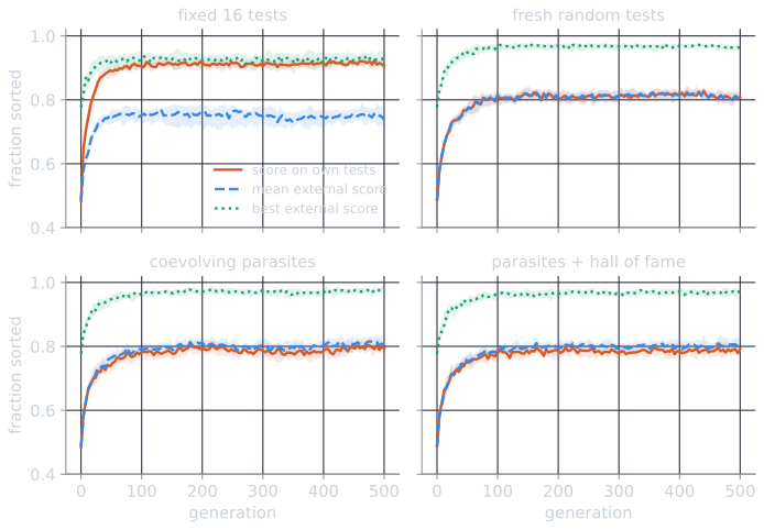
Four observations, all specific to this setup:
The fixed test set shows the measures diverging. The score on the 16 training tests rose from 0.48 to 0.91, while the mean external score reached 0.75 by generation 50 and then stayed between 0.74 and 0.76, and the median best network in the population reached 0.923 at generation 50 and never exceeded it. For the last 450 generations the algorithm reported a training score above 0.9 while making no progress on the actual problem. The fixed tests became the easy tests Hillis described: once the population sorted them, they no longer separated good networks from bad.
Under coevolution the relative score did not register the gains that were made. From generation 100 on, the population's mean score against its parasites stayed between 0.78 and 0.80, slightly below its mean external score, which was also nearly flat (0.79 to 0.81). Progress happened at the top: the median best external score rose from 0.960 at generation 100 to 0.978 at generation 500, and complete sorters appeared. The small gap between the two means shows that the parasites in this design made the tests only a little harder than random ones.
Coevolution found complete sorters most often, then lost them. A network that sorted all 247 inputs appeared in 16 of 30 coevolutionary runs (median first appearance at generation 202), against 6 with random tests and none with the fixed set. Only one run still had one at generation 500. Without elitism the algorithm keeps nothing by external merit, and a perfect sorter's relative score, the fraction of its one parasite's tests it sorts, is the same as that of any imperfect network that happened to meet a parasite it could handle. The relative fitness does not identify the best individual it has found.
The hall of fame did not help here. The variant found a perfect sorter in 7 runs, fewer than plain coevolution. One likely reason is that in this design it halves the tests drawn from current parasites, weakening the pressure that made coevolution effective. A single negative result in one setup says little about the method in general.
Where competitive coevolution fits
Competitive coevolution is worth its complications when no adequate fixed fitness function exists, because the space of opponents or test cases is too large to sample well and its informative part moves as the solutions improve. Games and test generation have this property. Where a fixed objective is available and cheap to evaluate exactly, coevolution adds noise and pathologies for no gain. Hillis's problem lies between the two: the objective is fixed and easy to state, but the informative tests change during the search, so coevolved tests can be more useful than random ones. Self-play in reinforcement learning and adversarial training of neural networks face the same question of how to measure progress against a moving opponent.
References
- Axelrod, R. (1980a). Effective choice in the prisoner's dilemma. Journal of Conflict Resolution, 24(1), 3–25.
- Axelrod, R. (1980b). More effective choice in the prisoner's dilemma. Journal of Conflict Resolution, 24(3), 379–403.
- Axelrod, R. (1997). The Complexity of Cooperation: Agent-Based Models of Competition and Collaboration, chapter 1. Princeton University Press. (Adapted from Axelrod, R. (1987). The evolution of strategies in the iterated prisoner's dilemma. In L. Davis (ed.), Genetic Algorithms and Simulated Annealing, 32–41. Pitman.)
- Eiben, A. E., and Smith, J. E. (2015). Introduction to Evolutionary Computing, 2nd ed., chapter 15. Springer.
- Hillis, W. D. (1990). Co-evolving parasites improve simulated evolution as an optimization procedure. Physica D: Nonlinear Phenomena, 42(1–3), 228–234.
- Pollack, J. B., and Blair, A. D. (1998). Co-evolution in the successful learning of backgammon strategy. Machine Learning, 32(3), 225–240.
- Rosin, C. D., and Belew, R. K. (1995). Methods for competitive co-evolution: Finding opponents worth beating. In L. J. Eshelman (ed.), Proceedings of the Sixth International Conference on Genetic Algorithms, 373–381. Morgan Kaufmann.
- Rosin, C. D., and Belew, R. K. (1997). New methods for competitive coevolution. Evolutionary Computation, 5(1), 1–29.
- Sims, K. (1994). Evolving 3D morphology and behavior by competition. In R. A. Brooks and P. Maes (eds.), Artificial Life IV, 28–39. MIT Press.
- Tesauro, G. (1995). Temporal difference learning and TD-Gammon. Communications of the ACM, 38(3), 58–68.
- Watson, R. A., and Pollack, J. B. (2001). Coevolutionary dynamics in a minimal substrate. In L. Spector et al. (eds.), Proceedings of the Genetic and Evolutionary Computation Conference (GECCO-2001), 702–709. Morgan Kaufmann.