A genetic algorithm evaluates whole strings, one at a time. Yet a single evaluation says something about more than one string. If the 16-bit string 1011001110100101 scores well, that is a small piece of evidence that strings beginning with 1 score well, that strings with 11 in positions 7 and 8 score well, and so on for every pattern the string matches. John Holland's theory of the genetic algorithm (see the history of evolutionary computation) starts from this observation. It treats the algorithm as processing, in parallel and without being told to, a very large number of such patterns, and it asks how selection, crossover and mutation change their numbers from one generation to the next. The answer is the schema theorem (Holland, 1975), popularized by Goldberg (1989, ch. 2) and long the standard explanation of why genetic algorithms work.
This article states the theorem precisely, checks it against a running algorithm, and then describes what it does and does not explain. The algorithm it concerns is the simple genetic algorithm (SGA). The textbook treatment is in Eiben and Smith (2015, ch. 16).
Schemata
A schema (plural schemata) over binary strings of length $l$ is a string over the three symbols $\{0, 1, *\}$. The symbol $*$ is a wildcard. A binary string is an instance of a schema if it agrees with the schema at every position where the schema has a 0 or a 1. For $l = 6$, the schema $H = $ 1**0*1 has the instances 100001, 100011, 101001, and five others, all the strings with 1 in the first position, 0 in the fourth and 1 in the sixth. Geometrically, a schema is a hyperplane of the $l$-dimensional hypercube of binary strings, which is why the literature also speaks of hyperplane sampling. For $l = 3$ the picture can be drawn. The eight strings are the corners of a cube, and two corners are joined by an edge when they differ in one bit. A schema of order 1 such as 1** fixes one coordinate and is a face of four corners; a schema of order 2 such as *10 fixes two and is an edge of two corners; a schema of order 3 is a single corner; and *** is the whole cube.
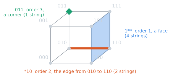
Two numbers describe a schema:
- The order $o(H)$ is the number of fixed positions, those holding a 0 or a 1. For
1**0*1it is 3. A schema of order $o$ has $2^{l - o}$ instances, so low-order schemata are large regions of the search space. - The defining length $\delta(H)$ is the distance between the first and the last fixed position. For
1**0*1the fixed positions are 1 and 6, so $\delta(H) = 5$. A schema with a single fixed position has defining length 0.
There are $3^l$ schemata. Each string is an instance of exactly $2^l$ of them, since each of its positions can either be kept or replaced by a wildcard. A population of $n$ strings therefore contains instances of at least $2^l$ and at most $n \cdot 2^l$ distinct schemata. The four 5-bit strings of Goldberg's (1989, ch. 1) $x^2$ example, 01101, 11000, 01000 and 10011, used in the simple genetic algorithm article, between them match 99 of the $3^5 = 243$ schemata on 5 bits, between the bounds of 32 and 128. The total falls short of 128 because schemata shared by several strings, such as ***** or ***0*, are counted once.
The theorem
Let $m(H, t)$ be the number of instances of $H$ in the population at generation $t$, let $f(H, t)$ be their average fitness, and let $\bar{f}(t)$ be the average fitness of the whole population of $n$ strings. The SGA builds generation $t + 1$ in three steps, and each step can be analyzed for its effect on $H$.
Selection. Fitness-proportional selection draws $n$ parents independently, each draw choosing string $x$ with probability $f(x) / \sum_y f(y)$. The expected number of parents that are instances of $H$ is then exactly
$$n \cdot \frac{m(H, t)\, f(H, t)}{n\, \bar{f}(t)} = m(H, t)\, \frac{f(H, t)}{\bar{f}(t)}.$$
A schema whose instances are above average in the current population gains copies in expectation, and one below average loses them.
Crossover. One-point crossover, applied to a pair with probability $p_c$, cuts both parents at one of the $l - 1$ positions between bits, chosen uniformly, and swaps the tails. An instance of $H$ is guaranteed to pass the schema intact to one of its two children if the cut falls outside the stretch between the first and last fixed positions. Only $\delta(H)$ of the $l - 1$ cut points fall inside it, so the probability that the schema survives crossover is at least $1 - p_c\, \delta(H) / (l - 1)$. It is "at least" because a cut inside the stretch does not always destroy the schema: when the mate carries the same values at the fixed positions beyond the cut, the child is still an instance.
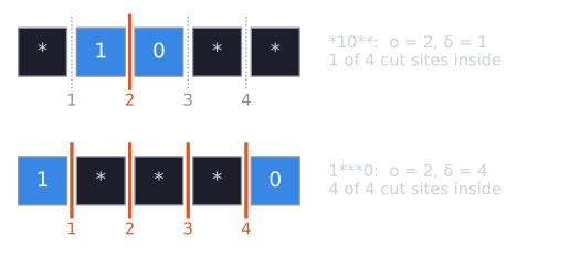
Mutation. Bit-flip mutation flips each bit independently with probability $p_m$. An instance survives if none of its $o(H)$ fixed positions flips, which happens with probability $(1 - p_m)^{o(H)}$.
Multiplying the three factors gives the schema theorem for the SGA:
$$\mathbb{E}\big[\, m(H, t+1) \mid P(t) \,\big] \;\ge\; m(H, t)\, \frac{f(H, t)}{\bar{f}(t)} \left[ 1 - p_c \frac{\delta(H)}{l - 1} \right] (1 - p_m)^{o(H)}.$$
Here $P(t)$ is the population at generation $t$, and the expectation is over the random choices of one generation. Since $(1 - p_m)^{o} \ge 1 - o\, p_m$, a weaker but simpler form follows, the one Goldberg (1989, ch. 2) made standard:
$$m(H, t+1) \;\ge\; m(H, t)\, \frac{f(H, t)}{\bar{f}(t)} \left[ 1 - p_c \frac{\delta(H)}{l - 1} - o(H)\, p_m \right].$$
In this form the left side is written $m(H, t+1)$, but it must be read as the expected value given the current population. The count in an actual run is a random variable and can fall below the bound, as the experiment below shows.
Three features of the statement matter for everything that follows:
- It is a lower bound. It counts only the instances that survive unchanged and ignores new instances created when crossover or mutation turns a non-member into a member.
- It concerns one generation. The quantities on the right, especially $f(H, t)$, change as the population changes, so the inequality cannot simply be iterated.
- $f(H, t)$ is the observed average fitness of the instances present in the population, not the average fitness of the schema over all $2^{l - o(H)}$ of its instances in the search space. Once selection has acted, the instances in the population are not a uniform sample of the schema, and the two averages can differ greatly.
The usual verbal summary is that short, low-order schemata with above-average fitness receive exponentially increasing numbers of trials in subsequent generations. The exponential part comes from treating the factor on the right as a constant $1 + c$ with $c > 0$, so that $m(H, t) \ge m(H, 0)(1 + c)^t$. That reading assumes the schema stays above average by a fixed margin, which it cannot do for long: as its instances spread, they make up more of the population, and $f(H, t) / \bar{f}(t)$ falls toward 1.
A worked generation
Every quantity in the theorem can be computed by hand for the four strings of Goldberg's $x^2$ example, with $p_c = 1$ and $p_m = 0.001$ as in the simple genetic algorithm article. The population has fitness values 169, 576, 64 and 361, mean $\bar{f} = 292.5$. Take three schemata:
| Schema | $o(H)$ | $\delta(H)$ | Instances | $m(H, 0)$ | $f(H, 0)$ | $f(H,0)/\bar{f}$ |
|---|---|---|---|---|---|---|
1**** |
1 | 0 | 11000, 10011 | 2 | 468.5 | 1.602 |
*10** |
2 | 1 | 11000, 01000 | 2 | 320 | 1.094 |
1***0 |
2 | 4 | 11000 | 1 | 576 | 1.969 |
The theorem is a product of three factors, and each can be evaluated in turn. Selection alone gives $m \cdot f(H)/\bar{f}$ expected instances in the mating pool. Crossover multiplies this by $1 - p_c\,\delta/(l-1) = 1 - \delta/4$, and mutation by $(1 - p_m)^{o}$. The last two columns compare the resulting bound with the exact conditional expectation, computed by enumerating every pair of parents, every cut site and every pattern of mutations, and with the count in the next generation of the hand-worked example in the simple GA article, whose children were 01100, 11001, 11011 and 10000:
| Schema | After selection | Crossover factor | Bound | Exact expectation | Hand-worked count |
|---|---|---|---|---|---|
1**** |
3.203 | 1 | 3.200 | 3.201 | 3 |
*10** |
2.188 | 0.75 | 1.638 | 2.230 | 2 |
1***0 |
1.969 | 0 | 0.000 | 1.751 | 1 |
(Rounded to three places.) The three rows show three degrees of looseness.
1****cannot be disrupted. With a single fixed position, no cut separates anything, and the bound misses the exact value only by the small chance that mutation turns a 0 into a 1 at the first position, which the bound ignores.*10**is disrupted less often than the bound assumes. Only a cut at site 2 can separate its fixed positions, and even then a child is an instance whenever the parent supplying the left part has a 1 at position 2 and the parent supplying the right part has a 0 at position 3. Weighted by selection probability, 69 percent of parents have the first and 86 percent the second, so a cut at site 2 yields an instance with probability $0.691 \times 0.856 = 0.592$, more than the 0.547 chance that a selected parent is an instance in the first place. The cut creates more instances than it destroys.1***0is rebuilt by every crossover. All four cut sites lie inside its defining length, so the bound is 0. But a child is an instance whenever it takes its first bit from a string beginning with 1 and its last bit from a string ending in 0, wherever the cut falls. These have selection probability 0.801 and 0.547, so each of the four children is an instance with probability 0.438, giving 1.752 expected instances before mutation and 1.751 after. In the hand-worked generation the single instance, 10000, came from crossing 10011, which is not an instance, with 11000 at site 2.
The weaker, linearized form of the theorem gives $1.969 \times (1 - 1 - 2 \times 0.001) = -0.004$ for 1***0, a negative bound on a count, true but empty. The example also shows that the theorem's quantities refer to a single generation: by the next one, 1**** has three instances out of four and its fitness ratio has dropped from 1.602 to $(625 + 729 + 256)/3 / 438.5 = 1.224$.
The bound in a running algorithm
The script tools/experiments/evolution/schema_check.py in the site repository runs an SGA and compares the bound with what actually happens. The algorithm has $n = 40$ strings of length $l = 16$, fitness $f(x) = 1 + (\text{number of ones in } x)$, roulette-wheel selection, one-point crossover with $p_c = 0.8$, and bit-flip mutation with $p_m = 1/16$. It tracks four schemata:
| Schema | Pattern | $o(H)$ | $\delta(H)$ | Survival factor $\left[1 - p_c \frac{\delta}{l-1}\right](1-p_m)^{o}$ |
|---|---|---|---|---|
| $H_1$ | 1*************** |
1 | 0 | 0.9375 |
| $H_2$ | 11************** |
2 | 1 | 0.8320 |
| $H_3$ | ****1111******** |
4 | 3 | 0.6489 |
| $H_4$ | 1**************1 |
2 | 15 | 0.1758 |
At each generation the script computes the bound, records the count actually produced in the run, and estimates the true conditional expectation $\mathbb{E}[m(H, t+1) \mid P(t)]$ by running 2,000 independent one-generation transitions from the same population. Over 30 seeded runs of 30 generations, these are the results for every generation in which the schema had at least one instance:
| Schema | Cases | Realized count below bound | Expected count below bound | Expected count / bound, median (IQR) |
|---|---|---|---|---|
| $H_1$ | 900 | 340 (37.8%) | 0 | 1.04 (1.02 to 1.06) |
| $H_2$ | 900 | 229 (25.4%) | 0 | 1.14 (1.11 to 1.19) |
| $H_3$ | 850 | 202 (23.8%) | 0 | 1.41 (1.30 to 1.63) |
| $H_4$ | 899 | 1 (0.1%) | 0 | 5.36 (5.13 to 5.72) |
"Expected count below bound" counts the cases in which the Monte Carlo estimate fell more than three standard errors below the bound. There were none, as the theorem requires. The rest of the table shows its two limitations.
The bound is loose, and its looseness depends on the schema. For $H_1$, which crossover cannot disrupt, the bound is within a few percent of the true expectation. For $H_4$, whose fixed positions are at the two ends of the string, the bound assumes that almost every crossover destroys the schema. At the first generation of run 0, $H_4$ had 12 instances with fitness ratio $f(H, t) / \bar{f}(t) = 1.088$, so the bound was $12 \times 1.088 \times 0.1758 = 2.30$, while the expected count was 12.47. A cut between the two fixed positions still leaves an instance among the two children whenever the mate has a 1 at either end, which in a random population is true of three strings in four. Crossover between two non-members can also create an instance. The bound ignores both.
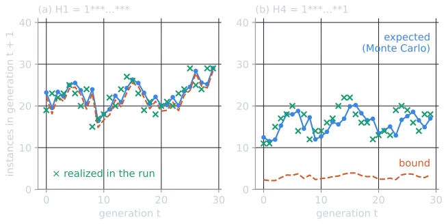
The same run shows why the "exponentially increasing trials" reading fails in practice. H1 was above average in every one of the 30 generations, with a fitness ratio between 1.007 and 1.117, yet its count did not grow exponentially: it wandered between 15 and 29 of the 40 strings. Selection adds $m(H,t)\,(f(H,t)/\bar{f}(t) - 1)$ instances in expectation, which in this run ranged from 0.14 to 2.7 and was below 1.3 in most generations. Mutation at the fixed position removes 6.25 percent of instances, one to two per generation, and returns some from the non-members. The realized count, meanwhile, missed its expectation by four or more instances in 5 of the 30 generations, and by 9 at generation 8 (15 instead of 23.96). Selection's push is smaller than the noise around it.
A single run is not an expectation. The count in the next generation is a sum of many random events, and its spread around the expectation is roughly of the order of the square root of the count. Where the bound is nearly tight, as for $H_1$, the realized count fell below it in more than a third of the generations. For $H_4$ the bound was so loose that only one realized count, in 899 cases, fell below it.
The same run also shows how little the bound promises when selection is weak, as fitness-proportional selection is on this fitness function (see selection pressure and premature convergence). At generation 0 of run 0, $H_1$ had 23 instances and fitness ratio 1.032, so the right side of the theorem was $23 \times 1.032 \times 0.9375 = 22.25$. The schema was above average, yet the bound predicted a decline, because the selective advantage of 3.2% was smaller than the 6.25% chance of a mutation at its fixed position. The true expectation, 23.21, was a slight increase, made up by mutations that turned non-members into members. With weak selection, as here, the verbal summary that above-average schemata grow does not follow from the bound at all.
Implicit parallelism
Since each string is an instance of $2^l$ schemata, each evaluation is in effect a sample of the fitness of every one of them. Holland called this implicit parallelism: a population of $n$ strings, processed by selection and recombination, works on far more schemata than it has strings. To make the claim quantitative, Holland counted the schemata that are processed "usefully", meaning those that are short enough to survive crossover with reasonable probability and represented often enough in the population for their counts to follow the theorem. For a population whose size is suitably matched to the string length, the count is of order $n^3$ (Holland, 1975; Goldberg, 1989, ch. 2). The $n^3$ figure was widely quoted as the reason genetic algorithms search efficiently.
The estimate depends on that particular relation between population size and string length. Bertoni and Dorigo (1993) redid the analysis for populations of size $n = 2^{\beta l}$, with $\beta$ a positive parameter. Holland's case corresponds to $\beta = 1$. They gave a lower bound on the expected number of processed schemata for every $\beta > 0$ and proved it tight up to a constant for $\beta \ge 1$. The $n^3$ figure is therefore a statement about one regime, not a general law about genetic algorithms.
There is also a more basic difficulty. Implicit parallelism counts schemata whose numbers change according to their observed average fitness in the population. Whether that observed average estimates anything useful about the schema as a whole is a separate question, and the theorem does not answer it. Grefenstette and Baker (1989) subjected implicit parallelism to an early critical examination, and Altenberg (1995) lists their paper among the early dissents from the standard account.
The building block hypothesis
The schema theorem says which schemata increase in number. It does not say how a genetic algorithm assembles a good complete string. Goldberg (1989, ch. 2) filled that gap with the building block hypothesis: short, low-order schemata of high fitness, the building blocks, are sampled, recombined by crossover and resampled, and by joining them the algorithm forms strings of ever higher fitness. On this account crossover is the engine of the algorithm, and the order of genes on the string matters, because building blocks are only "short" if the genes that work together sit close together.
The hypothesis is an empirical claim, not a consequence of the theorem. It fails, by construction, on deceptive problems, in which the short, low-order schemata with the highest average fitness point away from the global optimum. Trap functions are the standard examples, described in fitness landscapes. A deceptive problem is consistent with the schema theorem in every generation. The algorithm grows exactly the schemata the theorem says it should, and those schemata lead it to the wrong answer.
Critiques
What the theorem implies about performance. By the early 1990s several authors had questioned whether the theorem explains the power of genetic algorithms. Altenberg (1995) reviewed the objections. Mühlenbein (1991), as Altenberg quotes him, called the schema theorem "almost a tautology, only describing proportional selection", and observed that it ignores the question of why crossover builds better and better substrings. The theorem also holds for arbitrary subsets of the search space, not only for Holland's schemata: an analogous inequality can be written for any "predicate" on strings (Vose, 1991). It therefore singles out nothing special about schemata, and it holds equally for representations under which a genetic algorithm can do no better than random search.
Altenberg's own argument is that the theorem has no implications for how well a genetic algorithm performs. Performance depends on whether offspring of fit parents tend to be fit, a correlation the theorem neither states nor needs. His example is a needle-in-a-haystack function, with one high-fitness string and every other string equally poor. Once the needle has been found, every short schema containing it is above average and grows just as the theorem predicts, while crossover keeps producing hay. Using Price's covariance and selection theorem from population genetics, Altenberg derived the schema theorem and a theorem about the change in the population's fitness distribution from the same equation. The two differ only in the quantity measured, and only the second says anything about search performance.
Stochastic effects. Fogel and Ghozeil (1997) argued that the theorem cannot correctly estimate the expected proportion of a schema under proportional selection when fitness evaluation is noisy. Poli (2000) replied that the theorem remains correct when its quantities are treated as random variables and the statement is read as a conditional expectation given the current population, which is how it is stated above. The experiment above is a reminder of the distinction in its simplest form: the expectation obeys the bound, and individual runs need not.
Exact schema theorems. The theorem is an inequality because it ignores the creation of instances. Stephens and Waelbroeck (1997, 1999) replaced it with an exact equation for the expected proportion of a schema after selection and one-point crossover, which accounts for the reconstruction of a schema from pairs of shorter schemata to the left and right of the cut. In terms of an "effective fitness" that includes these effects, they recovered an exact version of the claim that schemata of above-average effective fitness grow. Their analysis also cut against the building block hypothesis: generically, the exact equation shows no preference for short, low-order schemata, and when reconstruction outweighs disruption, larger schemata are favored. Poli (2001) extended exact schema theory to genetic programming and variable-length genetic algorithms with one-point crossover. In a different line of work, Vose (1999) developed an exact model of the whole population for the SGA, in which the expected next population is a function of the current one and the state is the whole distribution of strings rather than a set of schemata.
What remains
The schema theorem, read correctly, is a true and modest statement: in one generation of the SGA, a schema's expected number of instances is at least its current number, multiplied by its observed fitness ratio and by the probability that crossover and mutation leave it intact. What it was once taken to mean, that a genetic algorithm efficiently processes $n^3$ building blocks and assembles them into an optimum, does not follow from it, and on deceptive problems the assembly of building blocks leads away from the optimum. The theorem retains value as a description of disruption: it explains why operators that disrupt less preserve more of what selection has found, and why the order of genes on the string matters under one-point crossover (the operators themselves are described in crossover and mutation operators). Modern theory of evolutionary algorithms relies mainly on other tools, such as exact population models and runtime analysis, of which the runtime result for the Trap function in fitness landscapes is an example. No theory of this kind can show that a genetic algorithm is better than other methods on all problems, for the reasons given by the No Free Lunch theorems.
References
- Altenberg, L. (1995). The schema theorem and Price's theorem. In L. D. Whitley and M. D. Vose (Eds.), Foundations of Genetic Algorithms 3, 23–49. Morgan Kaufmann.
- Bertoni, A., and Dorigo, M. (1993). Implicit parallelism in genetic algorithms. Artificial Intelligence, 61(2), 307–314.
- Eiben, A. E., and Smith, J. E. (2015). Introduction to Evolutionary Computing, 2nd ed., chapter 16. Springer.
- Fogel, D. B., and Ghozeil, A. (1997). Schema processing under proportional selection in the presence of random effects. IEEE Transactions on Evolutionary Computation, 1(4), 290–293.
- Goldberg, D. E. (1989). Genetic Algorithms in Search, Optimization, and Machine Learning, chapters 1 and 2. Addison-Wesley.
- Grefenstette, J. J., and Baker, J. E. (1989). How genetic algorithms work: A critical look at implicit parallelism. In J. D. Schaffer (Ed.), Proceedings of the Third International Conference on Genetic Algorithms, 20–27. Morgan Kaufmann.
- Holland, J. H. (1975). Adaptation in Natural and Artificial Systems. University of Michigan Press.
- Mühlenbein, H. (1991). Evolution in time and space: The parallel genetic algorithm. In G. J. E. Rawlins (Ed.), Foundations of Genetic Algorithms, 316–337. Morgan Kaufmann.
- Poli, R. (2000). Why the schema theorem is correct also in the presence of stochastic effects. In Proceedings of the 2000 Congress on Evolutionary Computation, vol. 1, 487–492. IEEE.
- Poli, R. (2001). Exact schema theory for genetic programming and variable-length genetic algorithms with one-point crossover. Genetic Programming and Evolvable Machines, 2(2), 123–163.
- Stephens, C. R., and Waelbroeck, H. (1997). Effective degrees of freedom in genetic algorithms and the block hypothesis. In T. Bäck (Ed.), Proceedings of the Seventh International Conference on Genetic Algorithms, 34–41. Morgan Kaufmann.
- Stephens, C. R., and Waelbroeck, H. (1999). Schemata evolution and building blocks. Evolutionary Computation, 7(2), 109–124.
- Vose, M. D. (1991). Generalizing the notion of schema in genetic algorithms. Artificial Intelligence, 50(3), 385–396.
- Vose, M. D. (1999). The Simple Genetic Algorithm: Foundations and Theory. MIT Press.