NEAT grows neural networks by mutation. The add-node mutation splits an existing connection in two and puts a new hidden neuron in the middle; the add-connection mutation links two neurons that were not linked. Either one usually makes a network worse before it makes it better. The new connection arrives with a random weight, and a new hidden neuron changes the function the network computes, adds weights that have not been tuned, and adds dimensions to the space that mutation must search. Meanwhile the rest of the population, smaller networks whose weights have had many generations to settle, keeps its fitness. Under ordinary selection the new structure is compared directly with them and removed. Stanley and Miikkulainen (2002, §3.2) put it plainly: because smaller structures optimize faster and adding structure usually lowers fitness at first, recently augmented networks "have little hope of surviving more than one generation", even when the structure they carry is what the task eventually needs.
NEAT's answer is to divide the population into species of similar networks and make networks compete mainly within their own species. A new topology starts a species of its own, or joins a small one, where it is compared with networks like itself and has time to tune its weights. This article describes how NEAT measures similarity, assigns genomes to species, shares fitness within species and allocates offspring, and how later implementations keep the number of species under control. It closes with an experiment on XOR that switches speciation off and varies the threshold that defines a species.
What speciation buys: the paper's ablation
Stanley and Miikkulainen (2002, §5) tested the claim by removing speciation from NEAT and running double pole balancing with velocity inputs. Removing it alone would have been uninformative, since without protection no structural innovation survives and every network stays minimal, so the nonspeciated version started from a population of random topologies, which supplies structural diversity without speciation. Over 20 runs it failed to find a solution within 1,000 generations 25% of the time, and when it succeeded it needed on average 25,600 evaluations, against 3,600 for full NEAT over 120 runs, with no failures. The authors traced the slowdown to convergence: within about 10 generations the population collapsed onto whichever topology happened to perform best at the start, on average one with about 5 hidden neurons, and smaller networks that would have optimized faster never got the chance (Stanley and Miikkulainen, 2002, §5.5). The same study found that each of NEAT's other components, starting minimally and crossover by historical markings, also mattered, and that they depend on one another: speciation can only measure similarity because historical markings line up genes.
The compatibility distance
Speciation needs a measure of how different two genomes are. For networks of different shapes this is hard in general, because two networks can compute the same function with their neurons in different orders (the competing conventions problem described in evolving neural network weights). NEAT sidesteps it with the innovation numbers on its connection genes. Two genes with the same innovation number descend from the same mutation, so lining genomes up by innovation number shows how much history they share.
When two genomes are aligned, genes present in both are matching. Genes present in only one are disjoint if they fall within the range of the other genome's innovation numbers and excess if they lie beyond it. The compatibility distance combines the three:
$$\delta = \frac{c_1 E}{N} + \frac{c_2 D}{N} + c_3 \overline{W},$$
where $E$ is the number of excess genes, $D$ the number of disjoint genes, $\overline{W}$ the average absolute weight difference of the matching genes (disabled genes included), $N$ the number of genes in the larger genome, and $c_1$, $c_2$, $c_3$ coefficients that set the importance of each term. The paper allows $N = 1$ when both genomes are small, fewer than 20 genes (Stanley and Miikkulainen, 2002, §3.3).
A worked example
Genome A has connection genes with innovation numbers 0 to 4; genome B has 0, 1, 2, 5, 6 and 7. Genes 0, 1 and 2 match. A's highest innovation number is 4, so B's genes 5, 6 and 7 lie beyond A's range and are excess ($E = 3$); A's genes 3 and 4 lie within B's range (B goes up to 7) and are disjoint ($D = 2$). The matching weights are $0.5$ and $0.9$, $-1.0$ and $-0.4$, and $0.2$ and $0.2$, so $\overline{W} = (0.4 + 0.6 + 0)/3 = 0.333$. Both genomes have fewer than 20 genes, so $N = 1$, and with $c_1 = c_2 = 1.0$ and $c_3 = 0.4$,
$$\delta = 3 + 2 + 0.4 \times 0.333 = 5.133.$$
That is above a threshold of 3.0, so A and B belong to different species. Had $N$ been the size of the larger genome, 6, the structural terms would have shrunk to $5/6$ and $\delta$ to 0.967; the small-genome rule keeps every structural difference significant while networks are small.
Now take genome C, a copy of A with every weight raised by 1.0 and one new connection gene, innovation 5. Then $E = 1$, $D = 0$ and $\overline{W} = 1.0$. With $c_3 = 0.4$, $\delta = 1 + 0.4 = 1.4$, and C shares A's species at threshold 3.0. With $c_3 = 3.0$ and threshold 4.0, the settings described next for the paper's hardest task, $\delta = 1 + 3.0 = 4.0$, which is not below 4.0, so C would found a new species. The weight coefficient decides whether networks of the same shape but different weights count as different species.
The script tools/experiments/evolution/speciation.py computes both examples with the distance function of the NEAT implementation in tools/experiments/evolution/neat.py.
The coefficients the experiments used
There are no standard values for $c_1$, $c_2$, $c_3$ and the threshold $\delta_t$. Each published experiment chose its own:
| Experiment | Population | $c_1$ | $c_2$ | $c_3$ | $\delta_t$ |
|---|---|---|---|---|---|
| XOR and double pole balancing with velocities (Stanley and Miikkulainen, 2002) | 150 | 1.0 | 1.0 | 0.4 | 3.0 |
| Double pole balancing without velocities (Stanley and Miikkulainen, 2002) | 1,000 | 1.0 | 1.0 | 3.0 | 4.0 |
| Robot duel, competitive coevolution (Stanley and Miikkulainen, 2004) | 256 per population | 1.0 | 1.0 | 2.0 | 3.0 at the start, then adjusted |
| HyperNEAT visual discrimination (Gauci and Stanley, 2007) | 100 | 2.0 | 2.0 | 1.0 | 6.0 at the start, then adjusted |
In the 2002 paper the hardest task, with the population of 1,000, raised $c_3$ to 3.0 "to allow for finer distinctions between species based on weight differences", since a larger population has room for more species, and raised $\delta_t$ to 4.0 to make room for the larger weight term (Stanley and Miikkulainen, 2002, §4.1). The authors describe the parameter values as found experimentally and performance as robust to moderate variations in them. The 2004 experiments fixed $N$ at 1 throughout. Extensions add terms: CPPN-NEAT, which evolves networks with mixed activation functions, adds a count of activation functions that differ between two genomes (Stanley, 2007; see CPPNs and HyperNEAT).
Assigning genomes to species
NEAT keeps an ordered list of species. Each species is represented by a random member from the previous generation. Every genome of the new generation is compared with the representatives in order and placed in the first species whose representative is within $\delta_t$ of it, so no genome belongs to two species. A genome compatible with no representative founds a new species and becomes its representative (Stanley and Miikkulainen, 2002, §3.3). Species left without members disappear.
Comparing with one representative, rather than with every member, makes assignment cheap: at most one distance per existing species for each genome. The paper notes that the average distance to all members of a species could be used instead, but that comparing with a single genome is sufficient in practice and takes constant time. The cost is some arbitrariness. A genome may be within $\delta_t$ of two representatives and is placed in whichever comes first in the list, and members of one species can be more than $\delta_t$ apart from each other, since each is only compared with the representative.
A worked assignment
Both effects appear in a small example, computed by tools/experiments/evolution/speciation_worked.py (Part 1) with $c_1 = c_2 = 1.0$, $c_3 = 0.4$, $\delta_t = 3.0$ and $N = 1$. Two species survive from the previous generation, in this order: S1, whose representative R1 has connection genes with innovation numbers 0 to 2, and S2, whose representative R2 has genes 0 to 4. Five genomes of the new generation arrive in order. Each row gives the distance to each representative tried, with the excess and disjoint counts and the mean weight difference $\overline{W}$ of the matching genes, rounded to three decimals:
| Genome | Innovations | To R1: $E$, $D$, $\overline{W}$, $\delta$ | To R2: $E$, $D$, $\overline{W}$, $\delta$ | Placed in |
|---|---|---|---|---|
| G1 | 0, 1, 2, 3 | 1, 0, 0.133, 1.053 | not tried | S1 |
| G2 | 0, 1, 2, 5, 6 | 2, 0, 0.133, 2.053 | not tried | S1 |
| G3 | 0, 1, 2, 3, 4, 7 | 3, 0, 1.000, 3.400 | 1, 0, 0.180, 1.072 | S2 |
| G4 | 0, 1, 2, 3 | 1, 0, 0.833, 1.333 | not tried (would be 1.060) | S1 |
| G5 | 0, 1, 6, 7, 8, 9 | 4, 1, 1.750, 5.700 | 4, 3, 1.750, 7.700 | new species S3 |
G3 has three genes beyond R1's largest innovation number, 2, so it is too far from R1 and goes on to R2, where it fits. G5 shares only genes 0 and 1 with either representative and founds a third species, becoming its representative for the rest of the generation. G4 shows the order effect: its distance to R2 would be 1.060, smaller than its 1.333 to R1, but R1 is tried first and is within the threshold, so G4 joins S1. And S1 ends with members that are not compatible with each other. G1 and G2 differ by one disjoint gene (3) and two excess genes (5 and 6), so $\delta(\text{G1}, \text{G2}) = 3.107$, and $\delta(\text{G2}, \text{G4}) = 3.280$; both pairs are farther apart than $\delta_t$, yet all three share a species because each is close to R1. A species is a set of genomes near one reference point, not a cluster in which every pair is similar.
Explicit fitness sharing and offspring allocation
Grouping alone does not protect anything; what matters is how species compete for places in the next generation. NEAT uses explicit fitness sharing (Goldberg and Richardson, 1987), described in general form in selection pressure and premature convergence. Each genome's fitness is divided by the number of genomes near it:
$$f'_i = \frac{f_i}{\sum_{j=1}^{n} \mathrm{sh}\big(\delta(i, j)\big)},$$
where the sharing function $\mathrm{sh}$ is 1 if $\delta(i, j)$ is below the threshold $\delta_t$ and 0 otherwise. The paper takes the denominator to be the size of $i$'s species, since species are already formed with the same threshold (Stanley and Miikkulainen, 2002, §3.3). Each species then receives a number of offspring proportional to the sum of its members' adjusted fitnesses. With every member's fitness divided by the species size, that sum is simply the species' mean fitness.
The effect is easiest to see with numbers. Suppose a population of 10 has three species:
| Species | Raw fitnesses | Raw total | Share of raw | Adjusted total (mean) | Share of adjusted | Offspring of 10 |
|---|---|---|---|---|---|---|
| S1 | 9, 9, 9, 8, 8, 8 | 51 | 0.586 | 8.5 | 0.347 | 3.47 |
| S2 | 12, 10, 8 | 30 | 0.345 | 10.0 | 0.408 | 4.08 |
| S3 | 6 | 6 | 0.069 | 6.0 | 0.245 | 2.45 |
Allocated by raw fitness, the large species S1 would take nearly 6 of the 10 places and the single network in S3 less than one. Allocated by adjusted fitness, the species with the best average, S2, takes the most, and S3, a lone network that might carry a new topology, gets more than two offspring even though its fitness is the lowest in the population. A species cannot grow merely by being large: as it grows, each member's share shrinks. Fractional allocations must be rounded to whole offspring; the paper does not say how, and neat.py uses the largest-remainder method.
Within each species, the lowest-performing members are then removed, and the population is replaced entirely by offspring of the remaining members of each species (Stanley and Miikkulainen, 2002, §3.3). Parents are normally chosen from the same species; in the paper's experiments a small fraction of matings, 0.001, crossed species.
Stagnation and elitism
Protection has to end somewhere, or species that will never improve would hold places indefinitely. The 2002 experiments used three rules (Stanley and Miikkulainen, 2002, §3.3 and §4.1):
- Species stagnation. If a species' maximum fitness did not improve for 15 generations, its networks were not allowed to reproduce.
- Population stagnation. In the rare case that the fitness of the whole population did not improve for more than 20 generations, only the top two species were allowed to reproduce, refocusing the search on the most promising regions.
- Elitism. The champion of each species with more than five networks was copied into the next generation unchanged.
Later work varied these rules. The 2004 robot-duel experiments, for example, prevented stagnation differently: the lowest-performing species over 30 generations old was not allowed to reproduce (Stanley and Miikkulainen, 2004, Appendix A). The paper's stagnation rule states no exception for the species holding the best network in the population, which can therefore be removed if the whole population stalls; neat.py departs from the rule by exempting that species.
Dynamic thresholds
The number of species depends on $\delta_t$ and on how far the population has diverged, and the second changes during a run. A threshold that gives a handful of species early on may give dozens later, when genomes have accumulated many disjoint genes, or one species that holds everything. Stanley and Miikkulainen (2004, §3.3) noted that the problem of choosing $\delta_t$ can be avoided by making it dynamic: given a target number of species, raise $\delta_t$ when there are too many and lower it when there are too few. In their robot-duel experiments the target was 10 species, $\delta_t$ started at 3.0, and it moved by 0.3 in the corresponding direction whenever the count was above or below 10 (Stanley and Miikkulainen, 2004, Appendix A). Gauci and Stanley (2007) used the same kind of scheme for HyperNEAT, with a starting threshold of 6.0, an adjustment of 0.3 and a target of eight species.
Library implementations made this optional. In neat-python, for example, the compatibility threshold is fixed by default; since version 2.1, setting target_num_species makes the threshold adjust after each generation toward that number of species, by threshold_adjust_rate (default 0.1) within the bounds threshold_min and threshold_max (defaults 0.1 and 100.0) (neat-python documentation). Its other defaults show the same rules as the paper under different names: max_stagnation defaults to 15 generations, while elitism within species and protection of the best species from stagnation (elitism, species_elitism) both default to 0, and survival_threshold lets the top 20% of each species reproduce.
A dynamic threshold does not guarantee a stable count. The course's soft-robot project steered its threshold toward a target of six species, and the count still swung between 1 and 29 over its final run. The project's report reads this as a control problem, with an adjustment too gentle to stop fragmentation and an emergency reduction that overshot.
Experiment: speciation on and off, and the threshold, on XOR
XOR is the paper's first test of NEAT: two inputs, a bias input and one output, starting from networks with no hidden neurons, so a solution requires growing at least one hidden neuron (Stanley and Miikkulainen, 2002, §4.2). The script tools/experiments/evolution/speciation.py runs the NEAT implementation in neat.py, with the paper's parameters for this task as defaults, under eight conditions, 30 seeded runs each, with a limit of 1,000 generations (150,000 evaluations). Fitness is the paper's $(4 - \sum \lvert \text{error} \rvert)^2$, and a network counts as a solution when all four outputs fall on the correct side of 0.5. "No speciation" puts every genome in one species, so there is no fitness sharing; the species-champion and stagnation rules still apply. "Random start" begins each genome with 1 to 10 hidden neurons and random links, as in the paper's nonspeciated ablation. The dynamic condition starts at $\delta_t = 3.0$ and moves it by 0.3 toward 10 species after each generation, the 2004 scheme. Evaluations, generations and the winner's hidden neurons are medians over the solved runs, with the interquartile range in brackets, rounded.
| Condition | Solved | Evaluations | Generations | Hidden neurons in winner | Species at generation 20 | Most species in a run |
|---|---|---|---|---|---|---|
| $\delta_t = 1.0$ | 30/30 | 4,587 [2,816, 8,709] | 31 [19, 58] | 2.5 [1.25, 3] | 119.5 | 123 |
| $\delta_t = 2.0$ | 29/30 | 14,609 [9,000, 22,955] | 98 [60, 154] | 5 [4, 6] | 77 | 94.5 |
| $\delta_t = 3.0$ (paper) | 30/30 | 8,348 [3,657, 14,587] | 56 [25, 97.5] | 4 [2, 4] | 16 | 21.5 |
| $\delta_t = 4.0$ | 27/30 | 11,617 [7,980, 21,218] | 78 [54, 142] | 4 [3, 6.5] | 6 | 13.5 |
| $\delta_t = 6.0$ | 26/30 | 23,804 [12,121, 45,994] | 159.5 [81.5, 307] | 4 [2, 7] | 1 | 6 |
| Dynamic, target 10 | 30/30 | 10,895 [7,357, 14,743] | 73.5 [50, 99] | 4 [3, 4.75] | 10 | 19 |
| No speciation | 12/30 | 24,523 [9,759, 47,401] | 163.5 [65, 317] | 3 [1, 7.25] | 1 | 1 |
| No speciation, random start | 29/30 | 1,367 [719, 9,168] | 10 [5, 62] | 9 [6, 10] | 1 | 1 |
Species counts are medians over the runs still going at that generation, and "most species in a run" is the median over runs of each run's maximum.
The clearest effect is the one speciation exists to prevent. Without it, starting from minimal networks, only 12 of 30 runs solved XOR within 1,000 generations. The share of genomes carrying at least one hidden neuron shows why: its median over the runs was 0.04 at generation 5, 0.05 at generation 10, 0.04 at generation 20 and still only 0.15 at generation 100. Add-node mutations kept happening, at a rate of 3% per offspring, but their products were not kept. With speciation at the paper's threshold the same share was 0.44 at generation 5, 0.83 at generation 10 and 0.93 at generation 20.
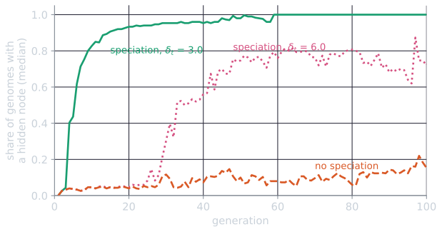
The low, nearly flat line without speciation is the arithmetic of the add-node mutation. Every generation about 3% of offspring receive a new hidden neuron, and the NEAT article works through an example in which splitting one connection drops a network's fitness from 8.87 to 6.21. With a single species, only the top 20% of the whole population reproduce, and a network that much worse than the median is rarely among them, so each generation's new hidden neurons are mostly gone in the next, and the share hovers around the rate at which they are created.
A threshold set too high has the same effect more slowly. At $\delta_t = 6.0$ the median number of species was 1 until generation 20, with the hidden-neuron share stuck at 0.05; protection arrived only when genomes had diverged enough to exceed the threshold, and 4 of 30 runs failed. At $\delta_t = 4.0$, 3 runs failed. Lower thresholds made many species: at $\delta_t = 1.0$ a single excess gene gives $\delta = 1.0$ when $N = 1$, which is not below the threshold, so almost every distinct topology was its own species, about 120 species in a population of 150 by generation 20. That setting was nonetheless the fastest of the speciated conditions on this task, with a median of 4,587 evaluations. XOR is small enough that spreading the population over many topologies costs little, and the result should not be read as a recommendation for harder problems. Between $\delta_t$ of 1.0 and 4.0 the interquartile ranges overlap, except that those of 1.0 and 2.0 just miss each other, and only the failures at 4.0 and 6.0 and without speciation stand clearly apart.
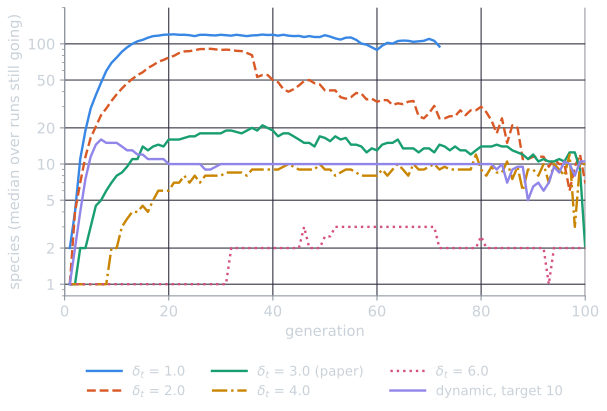
The dynamic threshold did what it was designed to do. The median number of species was 11.5 at generation 5 and 15 at generation 10, then held at about 10 from generation 20 onward, while $\delta_t$ itself wandered, from 2.1 at generation 5 to 5.7 at generation 20 and 3.7 at generation 100. It solved all 30 runs with a median of 10,895 evaluations, close to the fixed paper setting.
Inside one run
Medians hide how species come and go. The first run of the paper's setting (seed 0), which took 113 generations, made 156 species in all and never held more than 22 at once.
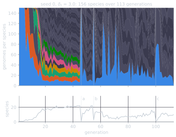
The founding species, every genome of which starts with the same three genes, holds the whole population until mutations accumulate enough structural differences, a sum of excess and disjoint genes of at least 3, to found new species. From generation 18 to 45 the count stays between 16 and 22 species of a handful of members each, which is what explicit fitness sharing produces when the species' mean fitnesses are similar. They were similar because the best network in every one of generations 10 to 45 scored within 0.01 of 9, the plateau described in the NEAT article, and at generation 45, 18 of the 21 species allowed to reproduce had a mean fitness between 7 and 9.
The three collapses have two different causes, which Part 3 of speciation_worked.py traces generation by generation. At (c), generation 100, the population had gone more than 20 generations without improving its best fitness, so the rule from the paper's footnote let only the top two species reproduce. The collapses at (a) and (b) are not a rule of the algorithm at all, but a side effect of the normalization in $\delta$ as this implementation applies it, with $N = 1$ exactly when both genomes have fewer than 20 genes. In both, the representative of the first species in the list had grown to 20 connection genes. At that size the small-genome exception no longer applies, $N$ becomes 20 instead of 1, and the structural terms of every distance to that representative shrink twentyfold: at generation 46, a genome of 7 genes compared with it had $\delta = 2.10$, where the same comparison with $N = 1$ gives 22.05, and at generation 55 a genome of 13 genes had 1.35 instead of 9.90. Since the first species is tried first, nearly every genome of the new generation fell into it. The paper says only that $N$ can be set to 1 for small genomes; applied as a hard cutoff, as here, that option makes $\delta$ jump at 20 genes. Implementations that divide by the genome size throughout, or never do, avoid the discontinuity, and whether a given implementation shows these collapses depends on that choice.
The random-start condition was by far the fastest, a median of 1,367 evaluations, because among 150 random networks with up to ten hidden neurons, some already compute or nearly compute XOR. Its winners carried a median of 9 hidden neurons, against 4 with speciation from minimal networks, so it bought speed with networks more than twice as large; the paper's random-start ablation, on the harder pole-balancing task, was 7 times slower than full NEAT (Stanley and Miikkulainen, 2002, §5.4). This is the article's own observation on one easy task: XOR rewards guessing a working network, and does not show the cost of searching in more dimensions than necessary that the paper measured. The paper also reports a mean of 4,755 evaluations for full NEAT on XOR over 100 runs (Stanley and Miikkulainen, 2002, §4.2), fewer than the median of 8,348 here; the NEAT article reproduces that experiment with the same implementation, which has to fill in details the paper leaves open.
Limits
Speciation in NEAT measures similarity of genomes, not of behaviour. Two networks with different histories can compute nearly the same function and be placed in different species, and two with shared history can behave very differently. Novelty-based methods, described in MAP-Elites and novelty search, measure diversity in behaviour instead. The threshold, coefficients and stagnation limits interact with the population size and the task, and the published values were chosen for particular experiments; a dynamic threshold replaces the choice of $\delta_t$ with the choice of a target count. And speciation is only one of NEAT's components: the paper's ablations show that it pays off together with growth from minimal networks and historical markings, not on its own.
References
- Gauci, J., and Stanley, K. O. (2007). Generating large-scale neural networks through discovering geometric regularities. In Proceedings of the 9th Annual Conference on Genetic and Evolutionary Computation (GECCO 2007), 997–1004. ACM.
- Goldberg, D. E., and Richardson, J. (1987). Genetic algorithms with sharing for multimodal function optimization. In Proceedings of the Second International Conference on Genetic Algorithms and Their Application, 41–49.
- neat-python documentation. Configuration file description. https://neat-python.readthedocs.io/en/latest/config_file.html (accessed November 2026).
- Stanley, K. O. (2007). Compositional pattern producing networks: A novel abstraction of development. Genetic Programming and Evolvable Machines, 8(2), 131–162.
- Stanley, K. O., and Miikkulainen, R. (2002). Evolving neural networks through augmenting topologies. Evolutionary Computation, 10(2), 99–127.
- Stanley, K. O., and Miikkulainen, R. (2004). Competitive coevolution through evolutionary complexification. Journal of Artificial Intelligence Research, 21, 63–100.